用 Amazon SageMaker HyperPod Data Capture 构建模型改进飞轮
Build a model improvement flywheel with Amazon SageMaker HyperPod Data Capture
Amazon SageMaker HyperPod 新增 Data Capture 能力,可在端点、负载均衡器、模型 Pod 三个独立层级把线上推理输入输出记录到 Amazon S3,对模型可用性零影响。文章以 Qwen2.5-3B-Instruct 家电客服路由模型为例,用 Athena 查询发现新产品盲区、SQL 策略打标后微调,验证部署后数据带来的准确率提升。
部署在 Amazon SageMaker HyperPod 上的基础模型会遇到任何预先整理的数据集都无法覆盖的输入:特定领域的专业术语、意料之外的格式、新产品以及不断变化的用户行为。如果没有生产推理数据的记录,团队就无法检测漂移、发现故障模式,也无法利用真实交互来改进模型。
Amazon SageMaker HyperPod 现在提供 Data Capture,这是一项内置功能,可将实时推理输入和输出记录到 Amazon Simple Storage Service(Amazon S3),分为三个独立层级,对延迟影响极小,且对模型可用性零影响。
在本文中,我们在单个 SageMaker HyperPod 集群上完整演示一个示例。一个家电支持路由器捕获其生产流量,Amazon Athena 查询揭示出一个新产品盲区,一条 SQL 策略为捕获的记录打上标签,基于这些数据进行微调让路由器学会了新产品。我们在模型部署前不可能存在的数据上测量了微调前后的准确率。推理算子在一个节点上提供模型服务,训练算子在另一个节点上运行微调。
本演练使用合成数据。脚本、清单、SQL、合成数据集和预期输出均可在配套的 GitHub 仓库中获取。
三层 Data Capture 架构
HyperPod Data Capture 提供三个独立层级,每个层级位于请求路径上的不同位置。你可以在同一个 dataCapture 块中开启任意组合。
| 第 1 层:SageMaker 端点 | 第 2 层:负载均衡器 | 第 3 层:模型 Pod | |
| 捕获内容 | 完整的请求/响应负载 | Application Load Balancer(ALB)访问日志字段:请求行、状态码、计时、客户端 IP、用户代理 | 完整的请求/响应负载以及事件元数据 |
| 管理方 | SageMaker 原生数据捕获 | ALB 访问日志 | HyperPod 推理算子(NGINX + OTel collector + S3 uploader sidecar) |
| 最适合 | 合规、Model Monitor、审计 | 低成本流量与错误率监控 | 调试、分析、训练数据收集 |
| 配置 | sagemakerEndpoint: — 采样百分比、输入/输出、AWS KMS |
loadBalancer: { enabled: true } |
modelPod: — 采样百分比、输入/输出、缓冲区、最大负载大小、AWS KMS、内容类型 |
第 1 层和第 3 层都存储完整负载,因此同时启用会将每条记录存储两次。将第 1 层用于合规和 Model Monitor,当你只需要流量元数据时使用第 2 层,当你打算使用负载时使用第 3 层。本文仅使用第 3 层。由于第 3 层记录完整负载,其中可能包含姓名、地址和订单号,因此请在这些数据成为训练数据之前加以保护。使用采样、AWS Key Management Service(AWS KMS)加密(kmsKeyId)、S3 生命周期规则以及个人身份信息(PII)脱敏(例如使用 Amazon Comprehend)。
先决条件
- 由 Amazon Elastic Kubernetes Service(Amazon EKS)编排的 SageMaker HyperPod 集群,已安装推理算子(为模型部署设置 HyperPod 集群)和训练算子 EKS 附加组件
amazon-sagemaker-hyperpod-training-operator(安装训练算子)。 - 两块可用的 NVIDIA GPU,一块用于服务,一块用于训练。我们使用
ml.g6e.8xlarge进行服务,使用ml.g6e.xlarge进行训练(各配备一块 48 GB NVIDIA L40S)。服务 Pod 在其端点生命周期内一直占用其 GPU,因此如果只有一块 GPU,训练 Pod 将保持Pending。 - 为集群配置了
kubectl。 - 同一区域中的 S3 存储桶。
确认两个 operator 均已安装。该命令返回两行:
kubectl get crd | grep -E 'inferenceendpointconfigs|hyperpodpytorchjobs'
hyperpodpytorchjobs.sagemaker.amazonaws.com                         2026-09-21T10:57:14Z
inferenceendpointconfigs.inference.sagemaker.aws.amazon.com         2026-08-06T11:58:53Z
解决方案概述
下图展示了在单个 SageMaker HyperPod 集群上执行该演练的五个步骤:将每个请求和响应捕获到 Amazon S3,使用 Athena 分析捕获数据,用 SQL 策略为其打标签,在第二个 GPU 上使用训练 operator 进行微调,并在捕获仍开启的情况下并排重新部署。
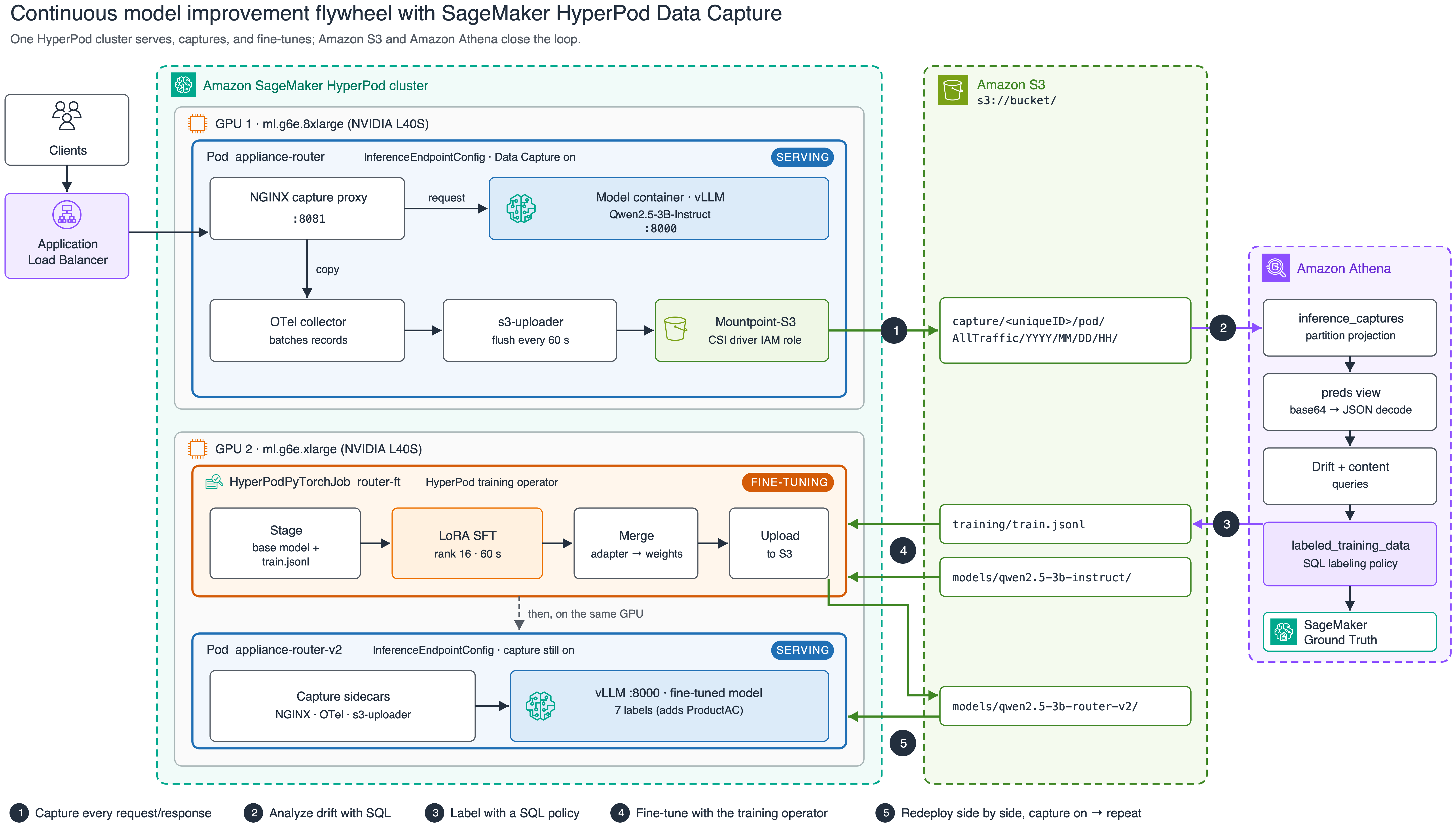
图 1:在单个 SageMaker HyperPod 集群上的五步飞轮,从捕获到 Athena 分析、打标签、微调以及重新部署
推理 operator 会向模型 Pod 添加三个 sidecar。每个经过 NGINX 代理的请求都会被复制到 OpenTelemetry collector,进行批处理后通过 Mountpoint-S3 卷写入 S3。Athena 会就地读取这些文件。训练 operator 在第二个 GPU 上以 HyperPodPyTorchJob 的形式运行微调,新模型由第二个同样开启捕获的端点提供服务。
步骤 0:设置变量
后续每个步骤都会读取这些变量。编辑第一个代码块,然后粘贴整个内容:
# --- edit these ---
export EKS_CLUSTER_NAME="my-hyperpod-eks"
export AWS_REGION="us-east-1"
export BUCKET="amzn-s3-demo-bucket"
export SERVE_INSTANCE_TYPE="ml.g6e.8xlarge"     # node type for the first endpoint
export TRAIN_INSTANCE_TYPE="ml.g6e.xlarge"      # node type for the fine-tuning job
# --- leave as-is ---
export AWS_DEFAULT_REGION="$AWS_REGION"
export ENDPOINT_NAME="appliance-router"
export MODEL_LOCATION="models/qwen2.5-3b-instruct"
export MODEL_V2_LOCATION="models/qwen2.5-3b-router-v2"
export TRAIN_SA="flywheel"                     # service account with S3 access via EKS Pod Identity
aws eks update-kubeconfig --name "$EKS_CLUSTER_NAME" --region "$AWS_REGION"
render() { python3 -c 'import os,sys; sys.stdout.write(os.path.expandvars(sys.stdin.read()))'; }
步骤 1:将基础模型暂存到 S3
我们使用 Qwen2.5-3B-Instruct,因为它足够小,可以在一分钟左右完成微调,并且能放在单个 L40S 上。
pip install -q huggingface_hub
python3 -c "from huggingface_hub import snapshot_download; \
  snapshot_download('Qwen/Qwen2.5-3B-Instruct', local_dir='qwen2.5-3b-instruct')"
aws s3 sync qwen2.5-3b-instruct "s3://${BUCKET}/${MODEL_LOCATION}/" --exclude ".cache/*"
步骤 2:IAM 权限
四个身份需要访问权限。有关策略语句,请参阅 Data capture for inference on HyperPod。
- Mountpoint-S3 CSI 驱动程序角色。 Tier 3 捕获通过 Mountpoint-S3 卷写入,驱动程序以其自己的 IAM roles for service accounts (IRSA) 角色进行身份验证,而不是以 Pod 的服务账户身份进行验证。它需要对捕获存储桶具有
s3:PutObject、s3:AbortMultipartUpload和s3:DeleteObject权限,如果你设置了kmsKeyId,还需要kms:Decrypt、kms:GenerateDataKey和kms:DescribeKey。如果缺少此权限,端点会保持健康且请求会成功,但不会出现任何捕获数据。请参阅 Mountpoint for Amazon S3 CSI driver。 - 推理 operator 执行角色。 它需要对捕获存储桶具有
s3:PutObject权限,如果你设置了kmsKeyId,还需要kms:Decrypt和kms:GenerateDataKey。捕获文件本身是通过 CSI 驱动程序角色写入的,因此当没有出现捕获数据时,请首先检查该角色。 - 训练 Pod 的服务账户(
$TRAIN_SA)。 通过 EKS Pod Identity 获得对基础模型和训练数据的读取权限,以及对合并模型的写入权限。 - Athena。 对捕获前缀的读取权限,以及一个查询结果位置。
启用数据捕获
接下来的三个步骤将部署开启 Tier 3 捕获的路由器,检查 Pod 是否运行捕获 sidecar,并确认记录到达 Amazon S3。
步骤 3:部署启用 Tier 3 捕获的模型
这就是该功能的全部内容:dataCapture.modelPod.enabled: true 代码块。其余部分都是普通的 vLLM 部署。
cat > endpoint.yaml <<'YAML'
apiVersion: inference.sagemaker.aws.amazon.com/v1
kind: InferenceEndpointConfig
metadata:
  name: ${ENDPOINT_NAME}
  namespace: default
spec:
  replicas: 1
  modelName: ${ENDPOINT_NAME}
  endpointName: ${ENDPOINT_NAME}
  instanceType: ${SERVE_INSTANCE_TYPE}
  invocationEndpoint: v1/chat/completions
  modelSourceConfig:
    modelSourceType: s3
    modelLocation: ${MODEL_LOCATION}
    s3Storage:
      bucketName: ${BUCKET}
      region: ${AWS_REGION}

  # >>> This is all you need to turn on Tier 3 data capture <<<
  dataCapture:
    s3Uri: "s3://${BUCKET}/capture/"
    modelPod:
      enabled: true
      initialSamplingPercentage: 100
      bufferConfig:
        batchSize: 50
        flushIntervalSeconds: 60
      payloadConfig:
        maxPayloadSizeKB: 1024

  worker:
    image: vllm/vllm-openai:v0.10.0
    modelInvocationPort:
      containerPort: 8000
      name: http
    modelVolumeMount:
      mountPath: /opt/ml/model
      name: model-weights
    args: ["--model", "/opt/ml/model", "--served-model-name", "${ENDPOINT_NAME}",
           "--port", "8000", "--max-model-len", "2048", "--gpu-memory-utilization", "0.90"]
    resources:
      requests: { cpu: "2", memory: 16Gi, nvidia.com/gpu: 1 }
      limits:   { nvidia.com/gpu: 1 }
YAML
render < endpoint.yaml | kubectl apply -f -
前面的 modelPod 代码块设置了 100% 采样并同时捕获输入和输出,这些是默认值。要调整它,请在 modelPod 下添加以下任意可选字段:
modelPod:
  enabled: true
  initialSamplingPercentage: 50          # capture 50% of requests (default 100)
  bufferConfig:
    batchSize: 100                       # records buffered per upload batch (default 10)
    flushIntervalSeconds: 60             # max seconds before a flush (default 60)
  payloadConfig:
    maxPayloadSizeKB: 1024               # truncate payloads larger than this (default: no limit)
  kmsKeyId: "arn:aws:kms:...:key/..."    # encrypt captures at rest
步骤 4:等待 Pod
启用捕获的 Pod 会运行四个容器:模型、sidecar-reverse-proxy(NGINX)、otel-collector 和 s3-uploader。模型容器和 Pod 的 app 标签都以 modelName 命名。
kubectl get pods -l app=$ENDPOINT_NAME -o custom-columns=\
'NAME:.metadata.name,READY:.status.containerStatuses[*].ready,CONTAINERS:.spec.containers[*].name,NODE:.spec.nodeName'
NAME                            READY                 CONTAINERS                                                              NODE
appliance-router-849f466476-4f5v8   true,true,true,true   appliance-router,s3-uploader,sidecar-reverse-proxy,otel-collector   hyperpod-i-0f3fe2684afd6a583
在我们的运行中,Pod 在 kubectl apply 之后大约五分钟就绪,其中大部分时间用于下载权重。
步骤 5:发送请求并确认捕获数据到达 S3
通过端口 8081 上的捕获代理发送推理请求,然后在刷新间隔之后列出捕获前缀。模型本身监听端口 8000。发送到该端口的请求会绕过代理,不会被捕获。
POD=$(kubectl get pod -l app=$ENDPOINT_NAME -o jsonpath='{.items[0].metadata.name}')
kubectl port-forward "pod/$POD" 18081:8081 >/dev/null 2>&1 &
sleep 5

curl -s http://localhost:18081/v1/chat/completions \
  -H 'Content-Type: application/json' \
  -d '{"model":"'"$ENDPOINT_NAME"'","messages":[{"role":"user","content":"my fridge is not cooling"}],"max_tokens":24}'

echo "Waiting for the capture buffer to flush..."; sleep 75
aws s3 ls "s3://${BUCKET}/capture/" --recursive | grep '\.jsonl$' | head
2026-09-28 15:47:14     634356 capture/20e4425092f90c7f/pod/AllTraffic/2026/09/28/15/28-15-47-12-999-ac31d31b-5156-46ad-9ccc-e8a040ab9ab2.jsonl
在 {s3Uri}/{uniqueID}/pod/{variant}/{YYYY}/{MM}/{DD}/{HH}/ 下你会看到一个或多个 .jsonl 对象。uniqueID 是按端点生成的。每一行都是一次推理,采用下面所示的 SageMaker 数据捕获格式。
捕获的记录格式
请求体和响应体以 base64 编码 的形式存储,如 encoding 字段所示,因此要读回它们需要先进行 base64 解码,再解析 JSON:
{
  "captureData": {
    "endpointInput":  { "observedContentType": "application/json", "mode": "INPUT",
                        "data": "eyJtb2RlbCI6ICJyb3V0ZXItZnJlc2giLCAidGVtcGVyYXR1cmUiOiAwLCAi...", "encoding": "BASE64" },
    "endpointOutput": { "observedContentType": "application/json", "mode": "OUTPUT",
                        "data": "eyJpZCI6ImNoYXRjbXBsLTctMTc5MDYxMDM2OS4wMDUtMjMxMiIsIm9iamVj...", "encoding": "BASE64" }
  },
  "eventMetadata": { "eventId": "26859f07-d60b-4683-94aa-d21e7f19e746", "inferenceTime": "2026-09-28T15:46:09Z" },
  "eventVersion": "0"
}解码后,endpointInput.data 是客户端发送的请求体,endpointOutput.data 是模型返回的响应。
场景:一个支持工单路由器遇上产品发布
部署的模型是一个面向家用电器零售商的支持工单路由器。它使用 vLLM 引导式 JSON 解码,将每张工单分类为六个类别之一:ProductFridge、ProductWasher、ProductOven、ProductDishwasher、ProductMicrowave,或兜底类别 Other。引导式解码意味着它只能返回带有这些标签之一的有效对象:
{"category": "ProductWasher", "confidence": 1}模型部署后,该零售商推出了自己的空调产品线——Arctis 系列(Arctis 9K、12K、Mini 等)。路由器没有针对它们的类别。它无法说“这是新的”。它只能选择它所知道的最接近的标签。除非每个请求和响应都被记录下来,否则证据会在响应返回的那一刻消失。
合成流量
我们生成了两个合成数据集:
- 生产流量:900 张工单,在 15 分钟内按顺序通过捕获代理重放,使用路由器最初的六标签提示词。前 400 张出现在发布之前,未提及任何空调。在剩余的 500 张中,Arctis 工单的占比从 15% 攀升至 55%。
- 评估集:280 张带标签的工单,每个类别 40 张,包括新的
ProductAC。它按内容留出:它使用的症状、句子模板和 Arctis 型号名称从未出现在流量中。
每个生产请求如下所示(系统提示词已缩写):
{"model": "appliance-router", "temperature": 0, "max_tokens": 40,
 "messages": [{"role": "system", "content": "You are a support-ticket router for a home-appliance retailer. ... category is one of: ProductFridge, ProductWasher, ProductOven, ProductDishwasher, ProductMicrowave, Other. ..."},
              {"role": "user", "content": "Hi, our Arctis 12K blows warm air since last week. Order #66759."}],
 "guided_json": {"type": "object", "required": ["category", "confidence"],
                 "properties": {"category": {"enum": ["ProductFridge", "ProductWasher", "ProductOven",
                                                      "ProductDishwasher", "ProductMicrowave", "Other"]},
"confidence": {"type": "number"}}}}要重放流量,请克隆随附的仓库,生成数据集,并将它们通过捕获代理发送。scripts/pod.sh 在模型容器内运行客户端,因此不需要负载均衡器或 DNS。客户端会打印 Athena 步骤使用的三个时间戳:RUN_START、LAUNCH_TS(发布后的第一张工单)和 RUN_END。
git clone https://github.com/awslabs/awsome-distributed-ai.git
cd awsome-distributed-ai/examples/use-cases/sagemaker-hyperpod-data-capture-flywheel
(cd data && python3 ../scripts/gen_dataset.py)
scripts/pod.sh $ENDPOINT_NAME drive /tmp/tickets_traffic.jsonl --seconds 900
RUN_START=2026-09-28 15:52:40
  sent 100/900
...
LAUNCH_TS=2026-09-28 15:59:20
...
RUN_END=2026-09-28 16:07:40
导出你的运行所打印的三个值,并等待一个刷新间隔:
export RUN_START="2026-09-28 15:52:40" LAUNCH_TS="2026-09-28 15:59:20" RUN_END="2026-09-28 16:07:40"
sleep 75    # one flush interval
用 Amazon Athena 揭示问题
离线基准在发布后看起来仍然没有变化,因为它们被冻结在过去。这种偏移只在捕获的生产流量中可见。本节展示数据科学家如何在不配置任何基础设施的情况下用 Athena 发现它。
步骤 6:设置变量并配置 Athena 辅助函数
export ATHENA_DB="flywheel_demo"
export ATHENA_OUTPUT="s3://${BUCKET}/athena-results/"
# Each endpoint writes under its own uniqueID. Pick the prefix whose captured requests name this
# endpoint, not whichever prefix sorts first (the Step 15 endpoint adds a second one).
for id in $(aws s3 ls "s3://${BUCKET}/capture/" | awk '/PRE/{print $2}'); do
  key=$(aws s3 ls "s3://${BUCKET}/capture/${id}pod/AllTraffic/" --recursive | awk '/\.jsonl$/{print $4; exit}')
  [ -n "$key" ] || continue
  model=$(aws s3 cp "s3://${BUCKET}/${key}" - 2>/dev/null | head -n 1 | python3 -c 'import sys, json, base64; r = json.loads(sys.stdin.readline()); print(json.loads(base64.b64decode(r["captureData"]["endpointInput"]["data"]))["model"])')
  if [ "$model" = "$ENDPOINT_NAME" ]; then export CAPTURE_LOCATION="s3://${BUCKET}/capture/${id}pod/AllTraffic/"; break; fi
done
echo "$CAPTURE_LOCATION"     # s3://<bucket>/capture/<uniqueID>/pod/AllTraffic/

# run_athena "<SQL>": runs one statement, prints tab-separated rows, and sets LAST_QID
run_athena() {
  local qid st
  qid=$(aws athena start-query-execution --query-string "$1" \
        --query-execution-context "Database=$ATHENA_DB" \
        --result-configuration "OutputLocation=$ATHENA_OUTPUT" \
        --output text --query 'QueryExecutionId') || return 1
  while :; do
    st=$(aws athena get-query-execution --query-execution-id "$qid" \
         --output text --query 'QueryExecution.Status.State')
    case "$st" in
      SUCCEEDED) break ;;
      FAILED|CANCELLED) aws athena get-query-execution --query-execution-id "$qid" \
          --output text --query 'QueryExecution.Status.StateChangeReason' >&2; return 1 ;;
    esac
    sleep 2
  done
  LAST_QID=$qid
  aws athena get-query-results --query-execution-id "$qid" \
    --output text --query 'ResultSet.Rows[*].Data[*].VarCharValue'
}
run_athena "CREATE DATABASE IF NOT EXISTS ${ATHENA_DB}"
步骤 7:向 Athena 声明捕获数据(两层)
第一层是信封。外部表描述每条记录的外层 JSON,对 year/month/day/hour 的分区投影将按小时的 S3 前缀映射到分区,无需爬网程序或 ADD PARTITION。data 字段被声明为普通字符串,因为它们是 base64 文本。
run_athena "
CREATE EXTERNAL TABLE IF NOT EXISTS inference_captures (
  captureData struct<
    endpointInput:  struct<observedContentType: string, mode: string, data: string, encoding: string>,
    endpointOutput: struct<observedContentType: string, mode: string, data: string, encoding: string>
  >,
  eventMetadata struct<eventId: string, inferenceTime: string>,
  eventVersion string
)
PARTITIONED BY (year string, month string, day string, hour string)
ROW FORMAT SERDE 'org.openx.data.jsonserde.JsonSerDe'
LOCATION '${CAPTURE_LOCATION}'
TBLPROPERTIES (
  'projection.enabled'='true',
  'projection.year.type'='integer',  'projection.year.range'='2026,2035',
  'projection.month.type'='integer', 'projection.month.range'='1,12', 'projection.month.digits'='2',
  'projection.day.type'='integer',   'projection.day.range'='1,31',   'projection.day.digits'='2',
  'projection.hour.type'='integer',  'projection.hour.range'='0,23',  'projection.hour.digits'='2',
  'storage.location.template'='${CAPTURE_LOCATION}\${year}/\${month}/\${day}/\${hour}/'
)"第二层是一个视图,对每条记录解码一次。from_utf8(from_base64(...)) 将负载转回 JSON。没有它,每次提取都会返回 NULL。工单是用户消息(messages[1],因为 messages[0] 是系统提示词)。模型的答案是响应 JSON 内的一个 JSON 字符串,因此需要第二次提取。
run_athena "
CREATE OR REPLACE VIEW preds AS
WITH decoded AS (
  SELECT CAST(from_iso8601_timestamp(eventMetadata.inferenceTime) AS timestamp) AS ts,
         from_utf8(from_base64(captureData.endpointInput.data))  AS req,
         from_utf8(from_base64(captureData.endpointOutput.data)) AS resp
  FROM inference_captures
  WHERE year = '${RUN_START:0:4}' AND month = '${RUN_START:5:2}' AND day = '${RUN_START:8:2}'
)
SELECT ts,
       json_extract_scalar(req, '\$.messages[1].content') AS ticket_text,
       json_extract_scalar(json_extract_scalar(resp, '\$.choices[0].message.content'), '\$.category') AS predicted_category,
       CAST(json_extract_scalar(json_extract_scalar(resp, '\$.choices[0].message.content'), '\$.confidence') AS double) AS confidence
FROM decoded
WHERE ts >= timestamp '${RUN_START}' AND ts < timestamp '${RUN_END}'
"
run_athena "SELECT count(*) AS n, count_if(predicted_category IS NULL) AS unparsed FROM preds"
n   unparsed
900 0
关于该视图的两点说明:
- 始终按分区过滤。Athena 读取原始 JSON,因此没有分区过滤的查询会扫描你曾经捕获过的每个对象。该视图过滤到一天,时间界限将其限制在我们的流量运行范围内:同一前缀还保存着步骤 5 的请求。
messages[1]假设一条系统消息后跟一条用户消息。 捕获的流量是客户端实际发送的内容,因此对于多轮或少样本请求,需要调整提取方式。
第 8 步:类别构成是否在变化?
run_athena "
SELECT date_trunc('minute', ts) AS minute, count(*) AS tickets,
       count_if(predicted_category = 'Other') AS other,
       round(100.0 * count_if(predicted_category = 'Other') / count(*), 1) AS other_pct
FROM preds GROUP BY 1 ORDER BY 1"
minute                   tickets  other  other_pct
2026-09-28 15:52:00.000       20      0        0.0
2026-09-28 15:53:00.000       60      3        5.0
2026-09-28 15:54:00.000       60      4        6.7
2026-09-28 15:55:00.000       60      4        6.7
2026-09-28 15:56:00.000       60      2        3.3
2026-09-28 15:57:00.000       60      1        1.7
2026-09-28 15:58:00.000       60      3        5.0
2026-09-28 15:59:00.000       60      9       15.0
2026-09-28 16:00:00.000       60     17       28.3
2026-09-28 16:01:00.000       60     14       23.3
2026-09-28 16:02:00.000       60     19       31.7
2026-09-28 16:03:00.000       60     21       35.0
2026-09-28 16:04:00.000       60     20       33.3
2026-09-28 16:05:00.000       60     32       53.3
2026-09-28 16:06:00.000       60     28       46.7
2026-09-28 16:07:00.000       40     26       65.0
(输出以制表符分隔。为便于阅读,我们在此处做了对齐。我们的运行将“数周”压缩到了 15 分钟。在生产环境中,请按 date_trunc('day', ts) 或 'week' 分桶。)
下图以柱状图展示每分钟路由到 Other 的工单占比,以折线展示累计占比,并标出了发布时刻。
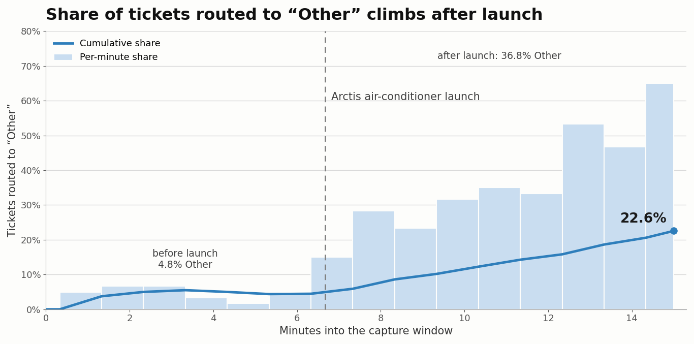
图 2:Arctis 发布前后,每分钟及累计路由到 Other 的工单占比
发布前,Other 每分钟保持在 7% 以下。发布当分钟跃升至 15%,并持续攀升,在最后三分钟达到 47–65%。图中的累计线仅达到 22.6%,因为它将发布后的工单与发布前的所有流量一起平均。这就是为什么应当将每分钟比率而非累计占比用于告警。
以发布时刻为界,整体类别构成如下:
run_athena "
SELECT IF(ts < timestamp '${LAUNCH_TS}', '1-before launch', '2-after launch') AS period,
       predicted_category, count(*) AS n
FROM preds GROUP BY 1, 2 ORDER BY 1, 3 DESC"
period           predicted_category    n
1-before launch  ProductFridge        91
1-before launch  ProductWasher        83
1-before launch  ProductDishwasher    74
1-before launch  ProductOven          74
1-before launch  ProductMicrowave     59
1-before launch  Other                19
2-after launch   Other               184
2-after launch   ProductFridge        84
2-after launch   ProductOven          66
2-after launch   ProductDishwasher    64
2-after launch   ProductWasher        58
2-after launch   ProductMicrowave     44
Other 从发布前的工单占比 4.8%(400 条中的 19 条)升至发布后的 36.8%(500 条中的 184 条),并成为最大的类别。
第 9 步:Other 桶里有什么?
run_athena "
SELECT word, count(*) AS freq
FROM preds CROSS JOIN UNNEST(regexp_extract_all(lower(ticket_text), '[a-z0-9-]{4,}')) AS t(word)
WHERE predicted_category = 'Other'
  AND word NOT IN ('this','that','with','from','have','since','week','help','need','again','time',
                   'month','second','take','look','someone','order','last','after','when','onto')
GROUP BY 1 ORDER BY 2 DESC, 1 LIMIT 10"
word      freq
arctis     141
unit        40
mini        33
cooling     30
link        30
lost        30
loudly      30
rattles     30
wi-fi       30
blows       28
Other 桶并非无关工单的混合。它被一个产品名 arctis 以及制冷设备的词汇所主导,这指向路由器没有对应标签的新类别。
第 10 步:规模有多大,模型的置信度能否标记出来?
在整个流量流中搜索该新产品,而不仅仅是 Other 桶:
run_athena "
SELECT IF(ts < timestamp '${LAUNCH_TS}', '1-before launch', '2-after launch') AS period,
       predicted_category, count(*) AS n
FROM preds WHERE regexp_like(lower(ticket_text), 'arctis|air condition')
GROUP BY 1, 2 ORDER BY 1, 3 DESC"
period          predicted_category    n
2-after launch  Other               164
2-after launch  ProductFridge        14
共有 178 条空调工单,占全部流量的 19.8%。它们在发布前均未出现。 它们分为两组:
- 164 条进入了
Other。 在六标签模式下,这是正确的答案:Other正是为此情况而存在。路由器没有坏。分类体系缺少一个类别,因此这些工单进入了通用队列,而不是支持该产品的团队。 - 14 条进入了
ProductFridge。 这些是真正的错误路由:冰箱团队现在收到了空调工单。
现在测试模型在这些已知错误路由上的置信度:
run_athena "
SELECT predicted_category, confidence, count(*) AS n FROM preds
WHERE regexp_like(lower(ticket_text), 'arctis|air condition')
GROUP BY 1, 2 ORDER BY 1, 2 DESC"
predicted_category  confidence    n
Other                      1.0  157
Other                      0.9    7
ProductFridge             0.95    1
ProductFridge              0.9    9
ProductFridge              0.8    2
ProductFridge              0.7    1
ProductFridge              0.0    1
在 14 条错误路由的工单中,有 10 条报告的置信度为 0.9 或更高。诸如“保留 confidence >= 0.9 的预测”这样的标注规则会保留 71% 的已知错误标签。这是因为 confidence 是我们要求模型写入的字段,而不是经过校准的概率。如果你需要真正的不确定性信号,请从 vLLM 请求 token logprobs,并读取类别 token 处的概率,而不是模型的自我报告。要为额外的负载大小做好预算,因为每次响应都会捕获 logprobs。
从诊断到带标签的训练数据
数据科学家不会手动标注数百条工单。相反,他们将 Athena 的发现写成一个标注策略:一个为每条捕获记录分配修正标签的 SQL 视图。我们将错误路由的空调工单重新标注为新类别。
第 11 步:标注策略
run_athena "
CREATE OR REPLACE VIEW labeled_training_data AS
WITH t AS (SELECT ticket_text, predicted_category, lower(ticket_text) AS txt FROM preds)
SELECT ticket_text, predicted_category,
  CASE
    -- 1. The new class, identified by keyword evidence, not by what the model predicted
    WHEN regexp_like(txt, '\\barctis\\b|air condition|\\bac unit\\b|mini split')
     AND NOT regexp_like(txt, 'fridge|refrigerat|freezer|washer|\\boven\\b|\\brange\\b|dishwasher|microwave')
      THEN 'ProductAC'
    -- 2. Keep the production decision when nothing hints at the new product
    WHEN NOT regexp_like(txt, '\\barctis\\b|air condition|\\bac\\b|mini split')
      THEN predicted_category
    -- 3. Mixed signals: send to human review (Amazon SageMaker Ground Truth)
    ELSE NULL
  END AS corrected_category
FROM t"双反斜杠(\\b)是双引号字符串内的 shell 转义。Athena 收到的是 \b,即正则表达式单词边界。
检查该策略生成了什么:
run_athena "
SELECT coalesce(corrected_category, '(human review)') AS label, count(*) AS n,
       count(DISTINCT ticket_text) AS distinct_texts,
       count_if(corrected_category <> predicted_category) AS relabeled
FROM labeled_training_data GROUP BY 1 ORDER BY 2 DESC"
label               n    distinct_texts  relabeled
ProductAC         178               114        178
ProductFridge     161               110          0
ProductWasher     141                96          0
ProductOven       140                97          0
ProductDishwasher 138                95          0
ProductMicrowave  103                82          0
Other              39                 8          0
这种启发式方法之所以有效,是因为新类别清晰明确(可通过关键词识别)。对于模糊工单或重叠类别,NULL 行将路由到 Ground Truth 进行人工标注。
第 12 步:构建训练文件
导出带标签的视图并将其转换为 chat 格式的 JSONL。允许的类别集合现在包含 ProductAC,即重新部署后客户端将发送的同样七个标签的提示词。将其保存为 build_training_file.py:
cat > build_training_file.py <<'PY'
import csv, json, sys
CATS = ["ProductFridge", "ProductWasher", "ProductOven", "ProductDishwasher", "ProductMicrowave", "ProductAC", "Other"]
PROMPT = ("You are a support-ticket router for a home-appliance retailer. Route each ticket to the product it "
          'concerns. Respond with ONLY a JSON object {"category": "...", "confidence": <0-1>} where category is '
          "one of: " + ", ".join(CATS) + '. Use "Other" if the ticket does not clearly concern one of these products.')
n = 0
with open(sys.argv[1], newline="") as fin, open(sys.argv[2], "w") as fout:
    for row in csv.DictReader(fin):
        fout.write(json.dumps({"messages": [
            {"role": "system", "content": PROMPT},
            {"role": "user", "content": row["ticket_text"]},
            {"role": "assistant", "content": json.dumps({"category": row["corrected_category"], "confidence": 1.0})},
        ]}) + "\n"); n += 1
print(f"wrote {n} training examples -> {sys.argv[2]}")
PY

run_athena "SELECT ticket_text, corrected_category FROM labeled_training_data
            WHERE corrected_category IS NOT NULL" > /dev/null
aws s3 cp "${ATHENA_OUTPUT}${LAST_QID}.csv" labeled.csv --only-show-errors   # Athena's own CSV: header + proper quoting
python3 build_training_file.py labeled.csv train.jsonl
aws s3 cp train.jsonl "s3://${BUCKET}/training/train.jsonl"
wrote 900 training examples -> train.jsonl
使用 HyperPod 训练算子对捕获的数据进行微调
我们在为模型提供服务的同一集群上进行微调,使用第二块 GPU 上的 HyperPod 训练算子。第一个端点全程保持服务。
第 13 步:训练脚本
该脚本从 S3 下载基础模型和训练数据,并训练一个低秩适配(LoRA)适配器。损失仅在助手回合上计算,因此模型学会生成标签,而不是重复提示词。随后脚本将适配器合并回基础权重,使 vLLM 可以原样提供结果,并将合并后的模型上传到 S3。该作业通过 ConfigMap 将脚本挂载到训练 Pod 中。
cat > train.py <<'PY'
import os, boto3, torch
from datasets import load_dataset
from peft import LoraConfig, get_peft_model
from transformers import AutoModelForCausalLM, AutoTokenizer, Trainer, TrainingArguments

s3 = boto3.client("s3")
def split(uri): b, _, k = uri[5:].partition("/"); return b, k

# 1. Stage base model + training data from S3
bucket, prefix = split(os.environ["BASE_MODEL_S3"])
for page in s3.get_paginator("list_objects_v2").paginate(Bucket=bucket, Prefix=prefix):
    for o in page.get("Contents", []):
        dst = os.path.join("/work/base", os.path.relpath(o["Key"], prefix))
        os.makedirs(os.path.dirname(dst), exist_ok=True); s3.download_file(bucket, o["Key"], dst)
s3.download_file(*split(os.environ["TRAIN_FILE_S3"]), "/work/train.jsonl")
print("[stage] base model and training data downloaded", flush=True)

# 2. LoRA SFT, loss only on the assistant turn (the label), not the prompt
tok = AutoTokenizer.from_pretrained("/work/base")
def encode(ex):
    full = tok.apply_chat_template(ex["messages"], tokenize=False)
    prompt = tok.apply_chat_template(ex["messages"][:-1], tokenize=False, add_generation_prompt=True)
    ids = tok(full, add_special_tokens=False)["input_ids"]
    n = len(tok(prompt, add_special_tokens=False)["input_ids"])
    return {"input_ids": ids, "labels": [-100] * n + ids[n:]}
ds = load_dataset("json", data_files="/work/train.jsonl", split="train")
print(f"[data] {len(ds)} examples", flush=True)
ds = ds.map(encode, remove_columns=ds.column_names)

def collate(batch):
    m = max(len(b["input_ids"]) for b in batch)
    pad = lambda xs, v: [x + [v] * (m - len(x)) for x in xs]
    return {"input_ids": torch.tensor(pad([b["input_ids"] for b in batch], tok.pad_token_id)),
            "labels": torch.tensor(pad([b["labels"] for b in batch], -100)),
            "attention_mask": torch.tensor(pad([[1] * len(b["input_ids"]) for b in batch], 0))}

model = AutoModelForCausalLM.from_pretrained("/work/base", torch_dtype=torch.bfloat16, device_map="cuda:0")
model = get_peft_model(model, LoraConfig(r=16, lora_alpha=32, lora_dropout=0.05, task_type="CAUSAL_LM",
    target_modules=["q_proj", "k_proj", "v_proj", "o_proj", "gate_proj", "up_proj", "down_proj"]))
model.print_trainable_parameters()
Trainer(model=model, train_dataset=ds, data_collator=collate, args=TrainingArguments(
    output_dir="/tmp/ckpt", num_train_epochs=float(os.getenv("EPOCHS", "2")), learning_rate=1e-4,
    per_device_train_batch_size=8, bf16=True, logging_steps=10, save_strategy="no", report_to=[],
    warmup_ratio=0.1, lr_scheduler_type="cosine")).train()

# 3. Merge the adapter into the base weights (a plain model vLLM can serve) and upload it
model.merge_and_unload().save_pretrained("/work/out", safe_serialization=True)
tok.save_pretrained("/work/out")
bucket, prefix = split(os.environ["OUTPUT_S3"])
for f in os.listdir("/work/out"):
    s3.upload_file(os.path.join("/work/out", f), bucket, f"{prefix.rstrip('/')}/{f}")
print(f"[done] merged model uploaded to {os.environ['OUTPUT_S3']}", flush=True)
PY
kubectl create configmap router-train --from-file=train.py
第 14 步:提交 HyperPodPyTorchJob
cat > finetune-job.yaml <<'YAML'
apiVersion: sagemaker.amazonaws.com/v1
kind: HyperPodPyTorchJob
metadata:
  name: router-ft
  namespace: default
spec:
  nprocPerNode: "1"
  runPolicy:
    jobMaxRetryCount: 2
    cleanPodPolicy: All              # release the GPU as soon as the job finishes
    logMonitoringConfiguration:      # restart a job that never starts, or goes quiet mid-run
      - name: JobStart
        logPattern: '.*loss.*'
        expectedStartCutOffInSeconds: 1200
      - name: JobHangingDetection
        logPattern: '.*loss.*'
        expectedRecurringFrequencyInSeconds: 600
  replicaSpecs:
    - name: pod
      replicas: 1
      template:
        metadata:
          labels: { app: router-ft }
        spec:
          serviceAccountName: ${TRAIN_SA}        # EKS Pod Identity -> S3 read/write
          nodeSelector:
            node.kubernetes.io/instance-type: ${TRAIN_INSTANCE_TYPE}
          restartPolicy: Always                  # required by the operator; retries live in runPolicy
          containers:
            - name: pytorch
              image: vllm/vllm-openai:v0.10.0    # already has torch + transformers + boto3
              command: ["bash", "-c"]
              args:
                - pip install -q peft==0.14.0 datasets==3.2.0 hyperpod-elastic-agent==1.1.3 &&
                  hyperpodrun --nnodes=1 --nproc_per_node=1 /scripts/train.py
              env:
                - { name: BASE_MODEL_S3, value: "s3://${BUCKET}/${MODEL_LOCATION}/" }
                - { name: TRAIN_FILE_S3, value: "s3://${BUCKET}/training/train.jsonl" }
                - { name: OUTPUT_S3,     value: "s3://${BUCKET}/${MODEL_V2_LOCATION}/" }
              resources:
                requests: { cpu: "2", memory: 24Gi, nvidia.com/gpu: 1 }
                limits:   { nvidia.com/gpu: 1 }
              volumeMounts:
                - { name: scripts, mountPath: /scripts }
                - { name: work,    mountPath: /work }
                - { name: shm,     mountPath: /dev/shm }
          volumes:
            - { name: scripts, configMap: { name: router-train } }
            - { name: work,    emptyDir: {} }
            - { name: shm,     emptyDir: { medium: Memory, sizeLimit: 8Gi } }
YAML
render < finetune-job.yaml | kubectl apply -f -
kubectl logs -l app=router-ft -flogMonitoringConfiguration是训练算子的显著特性。如果启动后 20 分钟内没有出现loss行,或者运行中途日志静默 10 分钟而进程仍然存活,算子会重启作业,而不是让它白白消耗 GPU 时间。- 该作业在启动时安装三个 Python 包。训练节点需要出站互联网访问(例如通过 NAT 网关),从 Docker Hub 拉取
vllm/vllm-openai镜像也需要。在没有互联网出口的集群上,请将包烘焙到 Amazon Elastic Container Registry(Amazon ECR)中的自定义镜像里,并去掉pip install。
作业日志摘录:
{'loss': 0.2484, 'grad_norm': 3.387, 'learning_rate': 3.91e-05, 'epoch': 0.09}
{'loss': 0.018, 'grad_norm': 0.0037, 'learning_rate': 8.26e-05, 'epoch': 0.18}
...
{'loss': 0.0, 'grad_norm': 0.000105, 'learning_rate': 2.93e-07, 'epoch': 1.95}
{'train_runtime': 59.68, 'train_samples_per_second': 30.16, 'train_loss': 0.0123, 'epoch': 2.0}
[done] merged model uploaded to s3://amzn-s3-demo-bucket/models/qwen2.5-3b-router-v2/
[HyperPodElasticAgent] ... Transitioned from AgentState.RUNNING to AgentState.COMPLETED
kubectl get hyperpodpytorchjob router-ft -o jsonpath='{range .status.conditions[*]}=  {end}'
Created=True  Completed=True
在一块 L40S 上训练耗时 60 秒。秩为 16 的 LoRA 训练约 2990 万个参数,不到 31 亿参数模型的 1%。平均训练损失为 0.0123,每步损失在第一个 epoch 内就达到 0.0,这表明模型很容易记住 900 个模板化示例。在真实数据上,请留出验证集并提前停止。这里我们依赖留出的评估集。
第 15 步:并排部署微调后的模型,同时保持捕获开启
不要编辑正在运行的端点,而是从同一清单将新模型部署为第二个端点,部署到训练作业刚刚释放的 GPU 上。第一个端点会持续服务,直到你将客户端切换过去,因此重新部署不会造成停机,回滚只需将客户端指回第一个端点。
export ENDPOINT_NAME="appliance-router-v2" MODEL_LOCATION="$MODEL_V2_LOCATION" SERVE_INSTANCE_TYPE="$TRAIN_INSTANCE_TYPE"
render < endpoint.yaml | kubectl apply -f -
kubectl get pods -l app=$ENDPOINT_NAME -o custom-columns='NAME:.metadata.name,READY:.status.containerStatuses[*].ready,NODE:.spec.nodeName'
NAME                                  READY                 NODE
appliance-router-v2-c96594c5-fhs2x    true,true,true,true   hyperpod-i-0e0b756209b5e497a
新端点在其自己的 uniqueID 下写入捕获数据。由于 ENDPOINT_NAME 现在是 appliance-router-v2,重新运行第 6 步中的 CAPTURE_LOCATION 查找会找到该前缀,因此你可以将第二个 Athena 表指向它,用于下一轮分析。当你迁移客户端时,请在同一版本中更新端点、标签集和引导式 JSON 枚举。
衡量提升效果
我们对微调后的端点运行了同样的 280 张留出工单:
overall 280/280 = 100.00%
  ProductFridge      40/40
  ProductWasher      40/40
  ProductOven        40/40
  ProductDishwasher  40/40
  ProductMicrowave   40/40
  ProductAC          40/40
Other 40/40| 指标 | 微调前(发布时) | 微调后 |
| 留出准确率(280) | 235 (83.9%) | 280 (100%) |
ProductAC (40) |
0/40 — 全部路由到 Other |
40/40 |
Other (40) |
35/40 | 40/40 |
| 五个既有产品类别(200) | 200/200 | 200/200 |
| 手写探针(24,接下来描述) | 16/24 | 20/24 |
微调教会了路由器新类别,并且对五个既有类别没有造成回归。它还修复了发布前就存在的五个 Other 错误,这些错误被已发布的路由器发送到了 ProductFridge。
由于我们的评估集与训练数据来自同一生成器,我们还手工编写了 24 张探针工单,采用生成器从未产生的风格。微调后的模型得分为 20/24:
  MISS ProductFridge -> ProductAC: The cooling fan in my fridge is squealing.
  MISS Other -> ProductAC: When will the Arctis 12K be back in stock?
  MISS Other -> ProductAC: Can I get a quote to install central air in my house?
  MISS Other -> ProductAC: Do you price match the Arctis at other stores?
overall 20/24 = 83.33%
它能正确路由全部八个空调探针,但学到了两个捷径:“cooling”意味着空调,而任何提到 Arctis 的地方都意味着ProductAC,包括库存和比价问题。两者都来自训练数据:标注策略把每一张 Arctis 工单都送到了ProductAC,而捕获的流量中不包含任何售前问题。在新端点上开启捕获后,这些工单正是下一轮捕获要收集的内容。
捕获会增加多少延迟?
我们直接测量了这一点:同样的 400 个路由请求,从 pod 内部分别发送到端口 8000(无捕获)或端口 8081(经由捕获代理)。我们以 8 个并发请求运行了三轮,另加一轮串行:
| 路径 | 并发 | p50 | p99 | 吞吐量 |
| 直连 vLLM(8000),无捕获 | 8 | 200.7 ms | 249.4 ms | 39.1 req/s |
| 经由捕获代理(8081) | 8 | 200.0 ms | 249.8 ms | 39.1 req/s |
| 直连 vLLM(8000),无捕获 | 1 | 164.4 ms | 206.9 ms | 6.0 req/s |
| 经由捕获代理(8081) | 1 | 164.4 ms | 207.0 ms | 6.0 req/s |
并发为 8 的行是三轮的平均值。轮次之间的波动(p50 处 ±1 ms)大于两条路径之间的差异。
捕获数据的其他用途
推理数据落入 S3 后,同样的记录可以供给许多工作流:
- 改进模型:使用监督微调(如本文所示),将大模型的输出蒸馏到小模型,或构建偏好对用于直接偏好优化(DPO)。
- 理解模型:运行 Athena 分析(如本文所示),从真实提示构建黄金回归集,设置漂移告警,发现新兴意图,并检测格式错误的输出和拒答。
- 运营与治理:将模糊样本路由到 Ground Truth 进行标注,保留审计追踪(推荐 Tier 1),重放事件背后的确切输入,并分析流量和负载以进行成本归因。
成本考量
| 层级 | 大致成本影响 |
| Tier 1(SageMaker 端点) | 由 SageMaker 在端点处捕获。你需要为负载支付 S3 存储和请求费用 |
| Tier 2(ALB 访问日志) | 仅为日志文件支付 S3 存储费用 |
| Tier 3(模型 pod) | 每个 pod 共三个边车请求 250m CPU + 640 MiB(NGINX 代理 100m/128Mi,OTel collector 100m/256Mi,s3-uploader 50m/256Mi),外加负载的 S3 存储和请求费用 |
有两项成本随使用量增长:
- S3。我们的记录平均每个约 2.3 KB(9.0 MB 中有 3,955 条记录)。更长的提示和响应成本按比例更高。上传器每个 pod 每个刷新间隔写入一个对象,在 60 秒间隔下每个 pod 每天约 1,440 次 PUT。
- Athena 按扫描的数据量计费,因此务必按分区列过滤,并使用
CREATE TABLE AS SELECT(CTAS)查询将原始 JSON 转换为 Parquet,以便重复分析。
有关当前价格,请参阅 Amazon S3 定价 和 Amazon Athena 定价。
清理
为避免产生不必要的费用,请清理本演练中创建的资源:
kubectl delete inferenceendpointconfig appliance-router appliance-router-v2
kubectl delete hyperpodpytorchjob router-ft
kubectl delete configmap router-train
run_athena "DROP VIEW IF EXISTS labeled_training_data"; run_athena "DROP VIEW IF EXISTS preds"
run_athena "DROP TABLE IF EXISTS inference_captures"; run_athena "DROP DATABASE IF EXISTS ${ATHENA_DB}"
aws s3 rm "s3://${BUCKET}/capture/" --recursive
aws s3 rm "s3://${BUCKET}/athena-results/" --recursive
aws s3 rm "s3://${BUCKET}/training/" --recursive
aws s3 rm "s3://${BUCKET}/${MODEL_V2_LOCATION}/" --recursive
结论
在本文中,我们展示了如何使用 SageMaker HyperPod Data Capture 记录实时推理数据并将其转化为训练数据。捕获在三个独立层级可用,因此你可以:
- 收集真实世界的训练数据,且对服务延迟没有可测量的影响。
- 使用 Amazon Athena 大规模查询推理模式,无需管理基础设施。
- 将 Athena 诊断转化为可复现的 SQL 标注策略。
- 在采集到的生产数据上进行微调,并衡量硬性的前后提升。
- 与 HyperPod 训练算子和 SageMaker Ground Truth 集成,以完成循环的其余部分。
我们在一个家用电器支持路由器上完整运行了一轮循环。采集到的流量揭示了一个新产品盲区,而 SQL 标注策略将这些采集数据转化为训练数据。使用 HyperPod 训练算子进行的 60 秒 LoRA 微调在提供模型服务的同一集群上运行。它使新类别从 0% 提升到完全召回,且对任何现有类别都没有回归。这些训练数据在模型部署之前都不存在。
Data Capture 现已在带有推理算子的 SageMaker HyperPod 集群上可用。要开始使用,请将 dataCapture 部分添加到你的 InferenceEndpointConfig 或 JumpStartModel 资源中并部署。要在同一集群上闭环,请添加 amazon-sagemaker-hyperpod-training-operator EKS 插件。本演练的完整代码位于随附的 GitHub 仓库中。
有关更多信息,请参阅 SageMaker HyperPod 推理文档和 HyperPod 训练算子文档。
关于作者

Shantanu Tripathi
Shantanu 是 AWS 的软件开发工程师,拥有构建大规模 AI/ML 基础设施的经验。作为 Amazon SageMaker 的核心工程师,他参与设计和优化面向高性能 AI 工作负载的可扩展推理解决方案。他的更广泛经验涵盖分布式 AI 训练库、深度学习容器(DLC)、深度学习 AMI 和生成式 AI 解决方案。工作之余,他喜欢戏剧和游泳。

Roy Allela
Roy 是 AWS 的首席 AI/ML 专家解决方案架构师。他与 AWS 客户(从初创公司到大型企业)合作,在 AWS 上高效地训练和部署基础模型。他拥有微处理器工程背景。他热衷于计算优化问题和提升 AI 工作负载的性能。

Piyush Daftary
Piyush 是 AWS 的首席软件工程师,从事 Amazon SageMaker 工作,专注于为大型语言模型构建高性能、可扩展的推理系统。他的技术兴趣涵盖 AI/ML、数据库和搜索技术,专长于开发可大规模实现高效推理的生产级解决方案。他的工作涉及优化系统性能、实现智能路由机制,以及设计支持研究和生产工作负载的架构,并热衷于解决复杂的分布式系统挑战,让开发者和组织更容易获得先进的 AI 能力。工作之余,他喜欢旅行、徒步和与家人共度时光。

Sean Archer
Sean 是 AWS 的软件开发工程师,为 Amazon SageMaker 构建 AI/ML 基础设施。他参与过支持可靠、可扩展模型部署的推理解决方案,以及 SageMaker HyperPod 集群的计算治理功能,帮助组织管理和分配大规模 AI 工作负载的计算资源。工作之余,他喜欢演奏音乐和旅行。
来源:AWS Machine Learning Blog · aws.amazon.com