研究称神经网络本身是干净的,叠加假说被误读
Neural networks are clean
作者在数月研究图像与语言模型的神经元和回路后提出,网络自身机制就是可读的构建单元,此前被视为多义性和叠加的经典证据被误读,实际多为一种递归泛化现象。作者称重新训练 InceptionV1 架构后,其最后一层 99-100% 的神经元易于解释,而初步审计 Qwen3-32B 时约 90% 的神经元极点只有一个主要功能。
作者以第一手实验重审多义神经元与叠加假说,给出递归泛化这一替代解释,可供理解可解释性研究走向。
译文尚不完整,完整内容请切换到原文。
简短版本
我认为关于神经网络的本质,我有个好消息。
在花费数月研究图像和语言模型中的神经元与回路之后,我开始相信,网络自身的机制就是其清晰可读的构建模块,而机制可解释性的前景可能远比我之前担心的要好。那些曾让包括我在内的领域内许多人相信网络会任意打包概念的多义性和叠加的经典证据,其实被误读了。看似随意的打包,大多是一种我称之为递归泛化的模式,这远没有那么令人担忧。这意味着我们可以直接研究网络,而不必先将其解开。神经网络本身已经是清晰的。
研究机制可解释性至少有两种途径。第一种是对网络本身进行快速的常规科学研究:观察网络的神经元和回路,研究它们之间的关系,观察数据如何在其中流动,并以智能体规模运行实验来检验解释。第二种则从一组假设的特征列表出发,试图将它们全部提取出来,设计越来越复杂的重建目标,并且通常忽略原始网络。
该领域始于第一种途径,后来退回到第二种,因为神经网络看起来像是一团乱麻。我们有多义神经元的经典例子——这是对看似承担多个不相关工作或看起来无法理解的神经元的统称。其中最著名的一个,在一个图像模型中,对猫脸和汽车前部都有反应。而早期领域模式生物 InceptionV1 的最后一层,似乎充满了随意的混合,以至于不清楚该如何研究它:几乎没有神经元是容易解释的。
对多义性的主流解释是叠加。这提出了一条新的学习原理:当神经网络的神经元不够用时,它不再将相关事物归在一起,而是开始将不相关的事物折叠在一起,仅仅因为它们不会相互干扰。结果就是一种结:网络本可以以许多几乎同样好的方式进行折叠,因此一个神经元将哪些事物归在一起,几乎不能告诉你任何信息。你必须先解开这个结,才能研究任何东西。在实践中,这意味着训练第二个模型——例如稀疏自编码器这样的分解——来近似网络展开后的样子,并转而研究那个模型。如果网络真的打了结,可能别无选择。
一个主要结果是,叠加性是对 InceptionV1 的错误解释。架构问题导致后面的层溢出。薄弱的可解释性工具放大了这些问题,使后面的层显得不连贯。此后,旨在帮助深层更好学习的架构改动产生了意想不到的效果,使它们更可解释。当我们最初研究 InceptionV1 时,我们在其最后一层几乎找不到可解释的神经元。但有了这些普通的改进,且模型大小或训练数据没有变化,最后一层中 99-100% 的神经元都易于解释,而且整个模型从头到尾都大致可读。这是我第一个觉得自己基本理解的非平凡神经网络;你可以在这里浏览它。我训练了它在 300 倍大小范围内的多个版本,它在每个尺度上都大致可读。空间较小时,网络不会把不相关的东西折叠在一起;它的神经元只是覆盖更粗粒度的概念,比如一个汽车神经元覆盖多种汽车。空间较大时,那个神经元会分化成许多具体的汽车。所以问题不在于存在第二种学习原理,而只是第一种原理的普通学习失败,而且很容易修复。
多义性和叠加性的经典视觉示例也是错误的。2019 年,Chris Olah 和我找到了最初在 Zoom InZoom In: An Introduction to Circuits
Olah, C., Cammarata, N., Schubert, L., Goh, G., Petrov, M. and Carter, S., 2020. Distill. References ↓ 中作为叠加现象引入的那个回路。它显示一个汽车特征似乎扩散到一组不相关的狗神经元中。那是我们展示的唯一一个,也是我见过的唯一一个。我们把它解读为网络把汽车放在一个高维隐藏处,供下游神经元读回。但没有任何东西读取那个组合。它没有隐藏任何东西;那是普通的泛化和组合。据我所知,没有人发表过第二个具有正确形状的回路。
现代语言模型也比人们普遍认为的可解释得多。Anthropic 的 Towards MonosemanticityTowards Monosemanticity: Decomposing Language Models With Dictionary Learning
Bricken, T., Templeton, A., Batson, J., et al., 2023. Transformer Circuits Thread. References ↓(2023 年)研究了一个小型单层模型,在其 14 分制的评分标准中,中位数神经元得分为 0,意味着评分者无法形成任何假设。我在 OpenAI 启动的自动化可解释性项目Language Models Can Explain Neurons in Language Models
Bills, S., Cammarata, N., Mossing, D., et al., 2023. OpenAI. References ↓(也是 2023 年)发现,按我们最宽松的标准,约 1.7% 的神经元可解释。
有了更好的工具和现代模型,情况看起来大不相同。在对 Qwen3-32B 的初步审计中,我们估计大约 90% 的神经元极点有一个主要职责,通常带有小的相关分支;另有约 7% 有两个相关职责;只有约 2-4% 尚未被理解关于这个数字的说明:具有单一职责的神经元比例会因你如何设定计数弱激活的阈值、深度、子回路密度,以及你把什么视为“一件事”而变化。
在这里,深入弱激活的程度是一个重要因素。下面有一节描述弱激活。它倾向于增加“相关事物”的数量,而不是神经元是否是对某种可读事物的判断。例如,特朗普神经元的弱激活会引入MAGA帽子和与他相关的人。泰坦尼克号神经元的弱激活会引入更一般的航行故事,或蒸汽机及那个时代的其他技术。
还有一个问题是是否要关注激活百分位数,或最强激活的比例。总的来说,我认为应该信任神经元学到的东西,它的自然稀疏性和激活范围等等。我以前大多不相信这一点!我有点反对试图在所有神经元之间标准化事物。如今百分位数更常见,我认为是因为它们更容易思考。
反过来也是如此。例如,当你查看泰坦尼克号神经元的“无关任务”时,它往往是在检测接下来是“船”。该工具错过了这一点,因为它在判断上下文时只向后看。当我们深入查看这些“无关任务”时,几乎总是这类情况。构建一个不完美的工具很容易。
总的来说,我认为得出单一分数实际上并没有那么重要。但当它被去掉时,早期审阅者感到没有锚点,连一个粗略的数字都没有。在我更仔细查看的集合中,考虑强激活,它更接近97%的非任意混合,但这些样本相对较小。
总的来说,将所有东西提炼成一个“清洁度”分数,应该被视为对神经网络所处状态的一个大致指向,而不是可以直接优化或过于严格把握的精确事物。这篇文章的很多内容是为了减少降维,根据每个神经元和回路的主题、深度、角色等区别对待它们。尽管如此,一个粗略的数字可能有用。
. 密集模型和专家混合模型似乎大致相似。我们在高达数万亿参数的模型中发现了类似结果,比如Kimi K3,配套论文将更详细地介绍。这些百分比将高维图景压缩成几个数字,而精确数字取决于你在哪里设定什么算作“一件事”的阈值——比如你是否将两种语言中密切相关的习语归为一类。我认为可解释性中没有什么重要内容取决于这个问题。更重要的是为什么事物首先共享一个神经元。
剩余的大部分明显多义性似乎源于一种我称之为递归泛化的模式。这很简单:随着神经元生长,它会像树枝长出子分支一样生出分支。例如,一个检测“iy”的神经元会逐渐检测“diy”,然后是“do it yourself”,而后者根本不包含“iy”。这个想法最早出现在我参与的一篇论文中被遗忘的一小节里,那篇论文叫多模态神经元人工神经网络中的多模态神经元
Goh, G., Cammarata, N., Voss, C., et al., 2021. Distill. 参考文献 ↓(2021年)。当时,我还没有观察过神经元在训练过程中的生长。现在这更容易了,而且在我见过的所有地方都成立。即使是原始的InceptionV1也没有打结。当我重新训练其原始架构时,它仍然会产生混乱的深层,并追踪我能找到的最难以辨认的神经元,结果发现它们在局部过度生长,进入了合理、相邻的领域。
所以多义性有两种解释,而这两种解释我都参与提出过。在某些方面,它们是相反的:泛化将相似的事物归为一组,而叠加将不相关的事物归为一组。叠加是该领域押注的解释,直到最近,我也是如此。但我现在认为递归泛化基本上是正确的。这样终究只剩下一个学习原则。它仍然是泛化,但事实证明泛化是分形的。这远没有那么令人担忧:事物的分组方式有可学习之处,而叠加中的两个项目则无可学习之处。而且由于泛化本身是分形的,我们的解释也可以如此:从基本解释开始,然后在想了解更多时放大。从这个意义上说,如果我们看得足够仔细,几乎整个网络都是可解释的,尤其是如果我们观察它在训练过程中是如何生长的。
为什么差距如此之大?我认为几个普通问题叠加在了一起。2023年的解释器模型无法运行猜想和测试的循环;工具和指标很弱,奖励的是能够模拟激活的解释,而不是正确的解释,而这两者往往不一致;没有人知道该期待什么样的语言神经元模式,人们普遍在寻找错误的东西;而且大多数研究使用的是小型或简化模型。从某种意义上说,那些模型确实已经没有空间了,这使得叠加成为自然的解释。但一个空间不足的网络不会改变学习原则;它的神经元只是变得更宽泛,就像小型视觉模型那样。一旦你知道该寻找什么,宽泛的神经元通常很容易分解。没有这种知识,再加上原始的工具,它们看起来就像任意的混合物。
可解释性有着惊人势头:就像拼图或填字游戏,你获得的任何理解都会开始约束系统的其余部分。起初,你盯着单个神经元。如果你无法理解它,其他帮助也不大:电路和归因图只能用你尚未理解的其他神经元来解释一个神经元。这会让起步变得困难。然而,一旦地图开始填充,进展就出奇地顺利。如果你不完全理解一个神经元的功能,你可以研究它连接的对象、它周围的生态系统,以及在专家混合模型中,它的专家专长于什么。就像拼图逐渐拼合,每一块都带来许多线索,而且它们结构良好、易于进行实验验证。这就是为什么近乎空白和基本填满都不是令人意外的状态;它们是自然的锚点。
拿一个追踪‘当廉价购买被证明比昂贵替代品更好用时产生的正义感’的神经元来说。追踪这种感受或社交线索的神经元是我们发现的最常见类型之一。想象一下,在不知道语言神经元模体、也没有电路可依赖的情况下发现这个神经元,因为邻近的神经元还很少被解释。大多数人类和智能体期望神经元通过激活来检测名词,但它们大多并不这样做。看看这个神经元最强烈激活的地方,你会看到一堆看似无关的逗号。
现在想象地图基本填满了。你知道许多神经元检测微妙的感受或社交语境,而且它们往往不是对承载感受的词语激活,而是对标点符号激活,比如逗号,模型在此总结句子的含义,或者对感受对预测后续内容至关重要的前一个词激活。因此,你转而阅读周围的句子,并检查它的引导效应(当你调高神经元时模型写什么),两者高度吻合。你查看上游它是如何构建的,下游它做什么,两者都吻合。你检查它的负极,什么会强烈推动它负向,发现同一线索的微妙变体,或社交语境结束的时刻。你可以运行特定测试,比如检查它对哪些商店品牌有反应。这些中的任何一个都可能推翻解释,但它们却不断指向同一处。理解这个神经元还能锐化更广泛的模体:在数千个微妙感受和社交语境检测器之后,你开始知道下一个会是什么样,这也是地图越填越快的原因之一。
这同样适用于工具。当你能看到网络的2%时,你无法判断工具哪里坏了;当你能看到大部分时,未解释的剩余部分直接指向它们。这就是我和一些同事如何在SwiGLU神经元中发现一个双负机制,据我们所知,此前无人注意到,而将许多神经元混合在一起的分解很可能会将其隐藏。
关于现代神经网络的坏消息是它们极其庞大。好消息是,庞大反而有帮助:随着地图填充,每个解释都受到周围一切的紧密约束,而更大的模型学习到更窄的神经元,这些神经元从一开始就更容易识别。
从这个意义上说,理解整个网络可能比只理解我们最关心的部分更容易。首先,除非你仔细研究过神经网络,否则很难知道如何像神经网络一样思考。例如,“欺骗”是一个有用的初始框架,但促成模型欺骗行为的构建模块很可能具有与对齐相关的微观结构,如果不深入进去观察,就很难了解。其次,针对一小组机制就像在只有一行的填字游戏上做文章。这是可行的,也可能奏效,但如果没有交叉线索,就很难知道你是否正确。解决整个问题——或者至少是这些机制所连接的网络的更广泛部分——可能更容易。
当我在现代卷积网络上运行这个过程时,它基本上奏效了。智能体可以绘制出神经元和回路,构建可探索的显微镜并对其进行探索,彻底测试解释,并追踪数十万个归因图。从未出现快速常规科学崩溃的时刻。我现在觉得自己基本上理解了这些模型,至少足以知道我会从哪里开始提出任何问题;最终,填字游戏被填满了。到目前为止,它在语言模型中也奏效,直到数万亿参数。由于规模庞大,这些还远未解决,但我对扩展这一过程持乐观态度。
所有这些让我回到一个旧的希望:直接理解神经网络,通过研究其机制以及它们之间流动的数据,而不必先试图修复或理清它。综合起来,这个论证有四个步骤。
- 网络使用一种学习原理,而不是两种(如果不是处处如此,也几乎足够多,以至于对研究无关紧要),因此开始对其进行常规科学研究没有障碍。
- 有了现代模型和工具,这项科学进展比大多数人预期的要好得多。
- 理解会累积,所以随着地图被填满,它会变得更容易。至少,网络自身的机制应该成为工具箱的一部分。
- 高度推测性:这可能就是我们所需的大部分,而可解释性可能比我们假设的要容易处理得多,也许在短期内就能实现。
这一直是深度学习总体的模式:在荒谬规模上的简单事物胜过聪明的事物。Rich Sutton 称之为苦涩的教训The Bitter Lesson
Sutton, R., 2019. Incomplete Ideas. References ↓。也许可解释性也有一个苦涩的教训:扩展常规调查胜过设计一种聪明的新分解方法。
一篇技术配套论文将提供关于语言模型神经元实验的更详细描述,例如我们发现关于现代非线性的不同机制,以及在不同深度出现哪些回路基序。这篇文章浏览了许多地方,并推测这一切可能指向何处。
汽车与动物
最著名的多义神经元是 InceptionV1 的 4e:55,它看起来像是猫和汽车的任意混合体。它被作为证据提出,说明神经元可能不是合适的研究单元,出现在该领域多篇被广泛阅读的论文中,从 2017 年的 Feature VisualizationFeature Visualization
Olah, C., Mordvintsev, A. and Schubert, L., 2017. Distill. References ↓ 到 Zoom InZoom In: An Introduction to Circuits
Olah, C., Cammarata, N., Schubert, L., Goh, G., Petrov, M. and Carter, S., 2020. Distill. References ↓。在我参与合著的 Zoom In 中,我们直截了当地说它“并不是在响应汽车和猫脸的某种共同点”。在 Multimodal Neurons 中我们非常接近了。我们问这个神经元是否可能在响应某种共享特征,“也许猫眼和车灯看起来相似”,然后根据特征可视化的胡须和镀铬判断它是“真正的 OR(cat, car)”。我们寻找共享形状是对的,但我认为我们低估了泛化的范围。共享特征是 V。我认为胡须误导了我们,因为泛化发生在高层模式内部。V 神经元确实接收了猫的回路,而特征可视化的任务是提高激活值,所以一旦它找到猫的路径,就会加上那条路径带来的一切。胡须也随之而来,即使神经元并不“想要”它们。在下游,汽车读取器确实通过 V 神经元得到了一点猫的信号,但它几乎到达不了输出:一个猫检测器单独激活作用很小,因为许多检测器协同工作,所以网络从不需要一个负权重来抵消它。要看到共享模式,你必须可视化神经元的输入有什么共同点,而不是神经元本身。
在看了几个月干净的神经元之后,我怀疑我们是否误读了一些早期著名的多义性和叠加的例子。典型的多义神经元似乎是显而易见的检查点,所以我打开了我看过数百次的猫和汽车图像网格,做了一件我从未做过的事:我花了几秒钟思考这可能是什么单一的东西。几乎立刻就很明显:这不是猫和汽车神经元,而是一个 V 形神经元。
我查看了它的回路连接:V 形火焰、消防船喷出的 V 形水柱、V 形狐狸脸。我查看了它的负极:一个 O,在 V 尖锐的地方是圆的。为什么猫和汽车的任意混合体需要如此强烈地连接到火焰?
inputs

4d:493 fox snout

4d:477 wolf face

4d:201 van front
4e:55
 Pointed
 generic
 Round
Round generic
readers

5a:94 flames

5a:352 coyote face

5a:317 martini glass
Pointed 使它激活
- dog
- fox
- cat
- car
- pool table
- bullet train
Round 使它负向
- dog
- dog
- snail
- golf ball
- tennis ball
- clock
然后我转向了我在2019年首次发现的典型叠加电路我是在构建我的第一个Circuits界面时发现的,当时它只有特征可视化和连接神经元之间的权重。然后我把它们拿给Chris Olah,问为什么汽车会这样进入这些狗。我们得出结论,它一定是在进行某种折叠,并称之为叠加。这是对我们所见现象的一种直观解释,所以并没有促使我们更深入地研究工具,否则会发现特征可视化奖励黑客和其他各种问题。它被置于高维空间似乎是一个合理的答案。。V神经元和这个电路是Zoom InZoom In: An Introduction to Circuits
Olah, C., Cammarata, N., Schubert, L., Goh, G., Petrov, M. and Carter, S., 2020. Distill. References ↓的两个主要例子,说明为什么其关于神经元的图景——即几乎每一个神经元只要你认真观察就能理解——可能“过于乐观”。
该电路似乎显示一辆汽车进入一群不相关的狗,仿佛狗是一种高维存储场所,汽车可以在需要时从中恢复。
但汽车并不是这样做的。汽车和狗被放在一起是因为共享的姿态。InceptionV1有超过一百个这样的广义姿态神经元,每一个都是对汽车、狗和其他物体共享姿态的独立干净检测器,据我所知没有人注意到它们。后面的层继续在此基础上构建,一直到模型结束。汽车并没有被存储在一个 obscure 的地方,也没有任何东西直接读出这种组合。恰恰相反:它继续分化为汽车专家和更精细的姿态。
部分原因是不了解广义姿态神经元,部分原因是我们用来渲染图像图标的技术——特征可视化——在更深的层中最终被奖励黑客了。其意图是找到一张最大化神经元的图像,但实现方式是通过梯度下降,它走最容易的路径,在InceptionV1中通常意味着狗。InceptionV1的训练数据中有很多狗,也有很多狗神经元,早期优化陷入其中,再也无法恢复。如果你甚至轻微地将其偏向顶部图像所走的自然路径,大多数是汽车,有些既是狗又是汽车,因为共享姿态。
我们以为的

任意存储场所
实际发生的
只是汽车
共享的汽车和狗姿态
人们很容易低估这种泛化,假设狗和汽车在一起只是因为空间不够。也许它“真的想要”单独的狗姿态和汽车姿态神经元,而一个空间更大的模型会将它们分开。确实,更大的模型往往有更窄的神经元,但当网络规模扩大时,它们可能以反直觉的方式做到这一点。
看看 DINOv2DINOv2: Learning Robust Visual Features without Supervision
Oquab, M., Darcet, T., Moutakanni, T., et al., 2023. arXiv:2304.07193. References ↓,它的规模是十倍以上,架构大约晚了十年,它有更多的姿态神经元,但其中许多仍然是泛化的。我在我看过的每一个视觉模型中,无论大小,都见过这种情况。
DINOv212× InceptionV1


ConvNeXt large4× InceptionV1


ConvNeXt medium1× InceptionV1


ConvNeXt small1/75× InceptionV1


人类和自动解释器似乎都强烈倾向于将神经元描述为名词组的检测器,比如猫和汽车,而不是描述为共享模式,比如 V。有时一个神经元确实对一组名词做出反应。但根据我的经验,它更常是一个共享模式,而这个神经元作为动词比作为名词更好理解。它的工作不是命名输入中的内容,而是画出下游神经元可以使用的区分:它在正极和负极分离出两种微妙的模式(V 与 O),并相应地将激活流推向不同的神经元。
我常常可以通过问自己来解开对某个神经元的理解:如果我完全不能使用名词组,我会如何向别人描述这个神经元?通常共享模式会立刻显现出来,并且很容易在更多名词组上测试(对于 V:新干线、台球桌)。我怀疑这是中层神经元中被错误归因的多义性的最大来源。我见过的许多将神经元称为多义的解释,在我看来都像是一个单一模式被描述为一串名词。
我们应该把一个意味着两三种东西的神经元视为一个具有几个分组含义的神经元。这种分组对网络来说可能不是问题:这些含义放在一起,因为从网络的角度来看,它们是相似的。这使得分组成为网络如何思考的线索,跟随它可以发现我们不知道的泛化,就像这里的猫和汽车一样。通常,额外的含义在仔细检查后也会消失,结果发现是次要的且很少激活。最后,一些表面上的含义只是我们的工具不好,这篇文章有几个例子:SwiGLU 的双重否定机制、一个未被读取的显著性旋钮使残差流难以可视化,以及我们刚刚看到的特征可视化中的奖励黑客。保持原始神经元的完整可以让这些错误保持可见,从而可以继续纠错。如果我们使用优化来获得更清晰的列表,我们可能会丢失许多这些线索。
显微镜错误的历史
在我看来,可解释性的故事在很大程度上就是发现显微镜下的东西比我们想象的更好。只是显微镜没有调好,而需要调整的东西往往相当微妙。
现代神经网络可解释性可以说是从特征可视化开始的,它渲染出一张合成图像,展示某个神经元最强烈响应的内容:那些著名的迷幻图片。有一段时间,它们看起来并不太好。你完全可以得出结论,这些神经元学到了某些东西,只是不够清晰。结果发现,这种方法缺少变换鲁棒性。一旦研究人员加入这一点,同样的神经元就变得清晰了。
但这只能让你深入模型到一定程度。在接近末端时,特征可视化又开始失效,原因有两个:我们在汽车回路中看到的奖励黑客行为,以及并不完全正确的正则化。修复它并不需要什么花哨的东西。对合理的设置做几处细微调整,现在我们就能更深入地观察网络。同样的神经元,更好的显微镜。
2009 风格20172026最强照片
中间层


最强照片


后层


最强照片


但这并不全是显微镜的功劳。模型也需要被调优。InceptionV1,这个领域早期的模式生物,在后层完全无法解释。一项估计称“据我所知,InceptionV1 的最后一层上基本上没有可解释的神经元”,这与我自己的记忆很接近,我可能会说 5%。它们当时看起来就是这样。
特征可视化数据集示例
据我所知,当时的主流解释是:相对于那里拥有的神经元数量和参数数量,需要表示的高层特征太多了,所以它开始把本不属于一起的特征任意打包,因为它们不会冲突。早期层是单义的,因为需要表示的早期层特征没有那么多。
但这不是正确的解释。这里有一个更现代的卷积网络,参数数量和数据集相同,但带有残差连接、LayerNorm 以及其他几项改进。最后一层很漂亮。
瓢虫 · 神经元 127
所以需要两件事。首先,神经网络需要学习得很好,使用由完全专注于这一目标、对可解释性毫无兴趣的人设计的架构。残差流就是一个例子:它被引入是为了帮助学习更深的神经网络,而且它似乎也有助于让更深层在概念上保持清晰,这两者可能有关。其次,我们需要足够强大的工具来清晰地看到它们。
InceptionV1 的最后一层曾是神经网络几乎从根本上不可解释的主要证据之一,因为它们学习的方式会重叠无关的混合特征。替换神经元似乎是唯一的选择。用那个时代的工具,我估计成功率在 5% 左右,其他人则认为约 0%。有了更好的可解释性工具(固定的特征可视化、可视化归因的方法等),在同一个网络上成功率更接近 50%。这都还是那个 2014 年的模型,其检查点和训练细节早已随时间丢失。用更合理的现代正则化重新训练同样的架构,成功率更接近 70%。在同样大小的 ConvNeXt 中,大约是 99%。它们可在此处探索。
递归泛化
所以我们已经证明最后一层是可以修复的。但在被修复之前,它在做什么?即使在架构改进之前,它也不是在任意地把东西拼凑在一起。当我们重新训练模型并观察一个神经元的形成时,它从黄色花朵开始,在有时包含狗的照片中。然后它沿着那些照片的每个侧面生长:朝向其他种类的自然、朝向像球这样的绿色物体,以及朝向没有任何花朵的狗。我看过的每一个神经元都是如此。改进后的架构显示出同样的模式,但程度要小得多。
每一行后面的灰色条带是它在神经元最强图像中所占的份额。
我们称之为递归泛化:一个神经元沿着不止一个轴泛化,通常先沿着一个轴,然后以局部容易跟随的方式向外发芽,但最终阻止它成为“单义”的。
例如,一个语言模型神经元响应“iy”,包括在“Miyazaki”中,然后响应“diy”,然后响应“do it yourself”,而后者根本不再包含“iy”。
在图像和语言模型中到处都有例子。就像一个地质学神经元泛化到 Cesium,一个地质学 JavaScript 库。
通常发生了什么非常明显,以至于很难知道是否就把它称为正常的泛化。就像一个敌人神经元,对一首关于敌人的俄语诗歌有反应。有时不太清楚但仍然合理。一个 Srinivasen 神经元也会轻微地对 UniProt 蛋白质数据库有反应。该项目有几个与之相关的 Srinivasen,但很难确定。
前 8 个激活
- String is a scalar string or 1-element string array, then STRSPLIT returns an array containing72
- 求 0 到 9 这些值的平均值:↵SPAWN, ’test_pipe’, UNIT62
- 设置此关键字以使“取消”按钮成为该对话框的默认选择。默认选择61
- Stage,↵ ModelExperimentalSceneMeshPrimitive,↵} 来自 "../../../Source/Cesium.js";↵↵describe("Scene59
- 地壳底部由原始结晶留下的富 KREEP 岩石 中 的 基 部 的 地壳 留下 的 原始 结晶 作用 的 的54
- 高地 比 北部 低地 更古老, 依据 是 覆盖 其上的 撞击 坑 数量 更多 的 撞击 坑 覆盖 可见54
- 在它们最后的日子里。 这段 戏剧性的 影像 拍摄于 12月 14日, 2054
- 在 夜空 中, 很 容易 看出 被称为 暗色 低地 平原的 区别 暗色 低地 平原 被称为54
按路线分组 前100名占比
- 月球和火星地壳44%来自L31火星、行星推动高地靠近暗面也是所在地于一个的太阳系中最大且最古老撞击特征之一,南极艾特肯盆地KREEP富含岩石位于地壳底部由地壳留下的原始结晶作用的
- 月球任务42%来自L28月球推动月球远处陨石坑地壳。但随着燃料即将耗尽,NASA决定让它们飞向月球附近的一座山月球使图像扭曲,LROC(Lunar勘测轨道器相机)现在
- 古老撞击,火星6%来自L30其他行星上的生命推动平原盆地火星存在。↵“3.4十亿年前一颗大型陨石引发了第一波海啸)↵换句话说,由于巨大的地狱内部压力积累作为撞击相当可能
- Cesium 和 IDL 代码8%来自L6像 Cesium 这样的名称推送.js对象软件以及降水率值,由此CesiumJS可以进而生成↵点Primitive对象。因为其中一些颜色数量,一旦初始化,不先退出ID就无法更改L。↵Colormaps定义
月球和火星地壳
高地、近侧和远侧、南极-艾特肯盆地
来自L31火星、行星L28月球
唤醒↑ L34中国的探月计划↑ L37深时
推向高地近侧暗色撞击
在夜空中,很容易看出两者的区别:被称为暗色低地平原的
月球任务
环绕、成像并撞击月球的航天器
来自L28月球L7月球,早期
唤醒↑ L36航天器、任务↑ L37撞击表面
推向月球远侧陨石坑卫星
但它们的燃料即将耗尽,所以NASA将命令它们撞击表面。↵因为它将
古老撞击、火星
赫拉斯、水手号峡谷、早期地球;较弱的喷发
来自L30其他行星上的生命L32大型火山
推向平原盆地火星
一周内拍摄的照片,聚焦于水手号峡谷西侧边界附近的一个陨石坑的VallesMarineris
Cesium 和 IDL 代码
CesiumJS 地球库和 IDL/ENVI 图像处理文档
通过L6像 Cesium 这样的名称L32软件文档中的数字
唤醒↑ L37JavaScript 库↓ L37太空新闻
推向.js对象软件视觉
要么 检测到 一个 空格 要么 检测到 一个 逗号。 在 这种 情况下, IDL 执行 一个 简单的 字符串 搜索
我们将在语言模型部分讨论这些递归泛化的分支以及它们有多重要。这里我们只想谈谈这个母题是什么。
我们最初在多模态神经元人工神经网络中的多模态神经元
Goh, G., Cammarata, N., Voss, C., et al., 2021. Distill. 参考文献 ↓中暗示了这一点,称它们为“联合特征”。在研究递归泛化数月后,直到我重新梳理该领域最著名的模型时,我才想起来。据我所知,没有人,包括我自己,提出过它可能是普遍的解释,例如解释 InceptionV1 最后一层出了什么问题。没有训练检查点,我们无法观察它的形成,但这个解释基本上是正确的。附录解释了我为什么认为新名称更准确。
叠加
递归泛化并不是一个特别大胆的解释,可以说它只是我们对普通泛化的预期。但对于多义性,也有人提出了一个更大胆得多的解释,一种新的学习原理。
我们随处可见的主要学习原理是泛化。在泛化中,事物因为共享的模式而被放在一起,这种模式放在一处很有用,因此可以在此基础上构建。在叠加中,不相关的事物因为不会相互干扰而被放在一起。这些有相反的预测:泛化应该是局部的,叠加应该是非局部的,因为它会希望非常不同的事物彼此靠近。
泛化会想要一个耷拉耳朵狗神经元,它可以被视为许多略微不同的耷拉耳朵以不同角度和种类放在一起。叠加会想要一个耷拉耳朵狗 + 拉丁诗歌神经元。
任意打包
不相关的事物共享一个神经元
泛化
相似的事物共享一个神经元
每个神经元 8 个事物
这里的定义变得纠缠不清。与叠加一起,Zoom InZoom In: An Introduction to Circuits
Olah, C., Cammarata, N., Schubert, L., Goh, G., Petrov, M. and Carter, S., 2020. Distill. References ↓ 引入了特征作为神经网络基本单元的概念。取决于你从哪个角度看,叠加要么意味着“特征多于维度”——即使是一个完全单义网络也会满足这一点,因为它的神经元会组合——要么意味着像上面那样的学习原理,有时应用于神经元所学的内容,有时应用于特征的所在之处。例如,InceptionV1 的第 4b 层基本上有单义神经元,对应车窗、车身和车轮等汽车部件,下一层将它们组装成汽车神经元 4c:447。在特征视角下,说“汽车特征”不仅存在于 4c:447 中,也存在于构建它的 4b 神经元的组合中,是合理的。因此,相邻层中有两个汽车特征,共享几乎完全相同的机制。在“特征多于维度”的视角下,第一个处于叠加状态,第二个可能不是。在非正式笔记 Distributed Representations: Composition & Superposition 的意义上,第一个是分布式的,但通过组合实现,第二个则完全不是分布式的。这就是为什么我觉得假设的特征难以思考,也是为什么我通常更喜欢具体的机制,比如神经元,以及具体的数据片段。
所以“叠加”本身也处于几种常见用法的叠加之中。我们关注应用于神经元等机制的学习原理,因为它是否成立对可解释性的好坏消息占比如此不成比例。它也相当容易测试:递归泛化和叠加预测的结果几乎相反,你可以观察一个神经元的成长,看看哪一种会发生。
在这篇文章中,当我说叠加时,我指的是这个版本,我们稍后会讨论“特征多于维度”的问题,我基本上不认为这是坏消息。
间隙的叠加
多义性往往更多是关于观察者的断言,而非关于神经元的。它说的是目前还没有好的解释。这可能有几个原因:
- 工具不好:我们的镜头或显微镜不够好
- 解释不好:由那些工具产生
- 学习不好:网络由于糟糕的架构、训练数据或其他原因而学得不好
- 递归泛化:在泛化过程中,神经元分叉出几个相关的方向
- 叠加:学习原理的变化,网络将不相关的事物塞进同一个神经元,因为它们很少碰撞。
多年来,我一直是叠加的坚定信徒。我开始研究语言模型神经元,并非出于对神经元或叠加的任何兴趣,而是因为我对智能体是否有研究品味感兴趣!我想看看它们在测试解释时是否会提出好问题,最初只是把神经元作为基线。我预期它们会遇到处于叠加状态中难以处理的特征碎片。那将为神经元的真实清洁程度产生一个新的基线,然后智能体可以继续使用一些更清洁的学习基。但它从未到来,因为神经元不断涌现,归结为一个简单的解释,做出了令人惊讶的预测,并且这些预测成立。
在一个前沿语言模型中,我发现了一个神经元,它主要在“pr”上激活,但也会对一堆 Base64 URL 字符串以及一些孟加拉语有反应。我以为这终于是一个任意的混合了。但解码那些 URL:是“pr”词。翻译那些孟加拉语:“pr”。
英语
请批pr准这个pr项目pr提案。
Base64
孟加拉语
প্রধানprodhanhead শিক্ষকshikkhokteacher প্রথমprothomfirst প্রশ্নটিproshnotiquestion করলেন।korlen.asked
在一个稠密的 Qwen 模型中,一位同事遇到了一个神经元,标准的 top-k 自动可解释性方法将其列为“多义逗号神经元”。但仔细观察后发现,它实际上追踪的是科罗拉多:电话号码、俚语,以及与其他科罗拉多神经元的连接。对它进行引导会让模型想要去徒步。那些逗号是它存储到目前为止科罗拉多上下文运行摘要的地方。一般来说,注意力似乎会聚集在标点符号上,我们称之为摘要母题。一旦你知道了这一点,许多类似的神经元就更容易理解了。
新工作,新城市,新租约,丹佛地址,303 区号,绿辣椒,周日野马队,红岩,蓝鸟粉雪日,萨尼塔斯步道口,十四峰。前三个逗号不激活;一旦丹佛出现,每个逗号都会激活,在绿辣椒之后达到最强。
我这个周末的计划是去图书馆复习考试。我还想去看望我的祖母,帮她做些园艺。
其他时候,我们只是没有足够的数据。起初我们没有包含长上下文,两段感觉就够了。但这意外地让所有长上下文神经元看起来都是多义的。
智能体所看到的
在另一个案例中,一个神经元看起来像一团任意的乱麻,没有任何东西强烈激活。事实证明,它在数页健康 SEO 垃圾内容中寻找特定迹象,而一旦我们有了足够广泛的数据集,它就可以理解了。
在数百个这样的案例中,没有什么动摇我对叠加的信念。它只是不断移动。如果强激活被清理干净,叠加就会转移到弱激活上,或者转移到神经元的组合上,或者转移到我还没看过的神经元上。或者也许跨越层本身。
但最终我开始思考这是怎么回事。除非这是某种戏剧性的扩展选择偏差案例,否则有些东西与早期的模型生物不符。于是我回过头去,最初的证据崩塌了,这便引出了这篇文章。
我现在认为,我之前把叠加当成了零假设,而它本应是最后的假设,因为它最激进、也最难检验。它看起来就像是不合理的东西。但糟糕的工具看起来也是这样(特征可视化奖励黑客),或者是你尚未追踪的递归泛化(“iy”神经元),或者是糟糕的架构(InceptionV1 的 5b),或者是你尚未理解的泛化(猫和车)。
I think part of what was going on was that superposition just felt right. Anthropic’s Softmax Linear UnitsSoftmax Linear Units
Elhage, N., Hume, T., Olsson, C., et al., 2022. Transformer Circuits Thread. References ↓ paper said as much in 2022: “In the mechanistic interpretability community, superposition is often treated as the default hypothesis simply because it seems intuitively more compelling than other explanations, but there is little evidence.”In the next sentence, the paper says its own results are moderate evidence for superposition. That evidence is circumstantial, in the paper’s own word: SoLU suppresses activations spread across many neurons, an extra LayerNorm restores performance, and after the LayerNorm a neuron’s weak activations looked less related to its main job, which the paper reads as features being smuggled through small activations. We read it as evidence about distributed representation in an architecture built to suppress it, rather than about neurons packing unrelated things together, which is the sense we care about. Telling the two apart in weak activations is hard even with today’s tools, since meaning shifts in every direction at once as activations weaken, and it was harder still in 2022, for all of us. The paper also notes that its discussion of superposition has been superseded by Toy Models of Superposition, which we address in the appendix. We bring it up not as a criticism of either paper, but because it’s the only place we know of where someone said plainly how little real-world evidence there was, and we think people still often assume there’s more than there is. To my knowledge, no one has found a superposition circuit in a real network since my original one, which was an error. I don’t see anything like it in real models, despite expecting to, and I think the bar for claiming it should be high, since it’s such a radical explanation and would be big news, terrible news, for how we should study neural networks.
Of course, this risks the opposite error, an explanation of the gaps: assuming every neuron must have a sensible story. Two things make it less worrying. First, each of the other causes can be tested. A better tool either resolves the neuron or it doesn’t; retraining with a better architecture shows whether learning was the problem; and recursive generalization can be watched as it grows, in small steps. Superposition’s only symptom is that something doesn’t make sense. Second, real explanations tend to be narrow and easily testable. Once you suspect a neuron is a Colorado neuron, steer it and see what it says. If a neuron fires for some narrow TV trope, the set of things that could count as that explanation is tiny, while “something that doesn’t make sense” covers everything outside it.
Also, we don’t have to force an explanation we don’t have. If a neuron might do a couple unrelated things and you’re not sure, it’s fine to say so. I think recursive generalization should be high on the list of things to suspect, and it’s easy to check if you have training checkpoints. I now think superposition should be far down the list.
Exploring Image Models
Small image models may seem obsolete, but I think they matter a lot to this question because we can see them so clearly. They're also where much of the original worry came from: there we saw what looked like high-resolution chaos, not low-resolution ambiguity. Language models are massive, we don't have tools like feature visualization which make our life easier, attention mixes different kinds of mechanisms together, and many of their motifs are surprising. As I showed above, even vision motifs can be counter-intuitive, and language is worse. Each one of these deficiencies can make a monosemantic neuron look polysemantic. If you're looking at a blurry image trying to figure out if it's a dog or a cat, the blur makes it harder, but it doesn't favor either answer. If you're looking at a blurry image and trying to decide if the image itself is blurry or if you're just looking badly, every flaw in your eyesight gets counted as blur in the image. If we want to study how neurons change with scale, compression pressure, activation strength, and depth, it's better to start where we can see clearly.
I trained three ConvNeXt models spanning roughly 300× in size: a small one with 92k parameters, a medium one with 7.06M (the same size as InceptionV1), and a large one with 28.6M. We’ll look at those, and also InceptionV1, to try to understand what neurons do in different situations, and try to find places packing may form.
How I Think About Neurons
I used to think of neurons as human-shaped nouns: one is a car, another is a curve. Now I think of them more as control flow. A neuron is less about what it sees than about what it does to the flow coming in, and often its job is to gate a region of the network. Seen this way, monosemanticity is almost the wrong question. A better one is what a neuron lets through and what it keeps out.
Pixels come in, and the network begins grouping and distinguishing things. Cars and dogs might be grouped together because they share a pose. Further along there are specific car detectors – for taxis, ambulances and the like – and they don’t want dogs. So a neuron in front of them acts as a gate: it responds positively to cars and negatively to dogs, and its negative side keeps the dogs out. The dogs go on to their own area, which doesn’t have to worry about cars. Later neurons build on this, specializing further: an ambulance neuron might have a taxi on its negative pole, and a taxi an ambulance. In a larger model, these distinctions can become finer still, separating one view of a taxi from another. Smaller models may stop at coarser distinctions, with something closer to a general “car” neuron.
Here’s a real sports car, followed through the last five blocks of our large model. Partway through, it’s grouped with other rectangular shapes, like tables and cabinets, against snakes and dogs. By the last block, the split is convertibles against station wagons.
The negative side of neurons matters almost as much as positives for understanding them, even in ReLU networks where the negative side is cut off. A neuron is built from votes: each input weight votes for its positive side or its negative side, and the votes add up before the nonlinearity. The negative side never gets gradient on its own, but the individual votes do whenever the neuron is on, so it’s shaped by learning too. The negative side’s meaning depends on context: when a neuron in the sports car’s path separates it from snakes and dogs, it isn’t calling cars and dogs opposites, just gating out things that were usefully grouped earlier. The negative side tells us what distinction matters at this point in the circuit, which also makes it a quick check on whether a grouping is real: the V neuron’s negative side is an O.
If we look at the last layer, we see high-level patterns and what they’re being distinguished from: taxis from ambulances, broccoli from cauliflower, and spoonbills from flamingos.
+Taxis


−Ambulances


+Broccoli


−Cauliflower


+Spoonbills


−Flamingos


+Toucans


−Hornbills


+Lighthouses


−Water towers


+Pretzels


−Bagels


+Wolves


−Huskies


+House cats


−Lynxes


+Mittens


−Socks


The two strongest images at each pole. The sign is the neuron’s own response, not its effect downstream. Neurons in the last block (stage3.block2): taxis 230, broccoli 829, spoonbills 1440, toucans 2021, lighthouses 1956, pretzels 1068, wolves 401, house cats 1637, mittens 63.
When we look at our smallest model, we see the neurons get coarser. Its last layer ends at cars, trains, and carts in one neuron, with boats, planes, and a water-based ox-cart, (which I didn’t know even existed), on its negative side. It’s still differentiating, but more coarsely, and it ends early.
+


−


What Neurons Do Under Pressure
Early layers in most vision models are monosemantic. As I understood it, the standard explanation is because there’s not that many early vision features that need to be represented. On its surface, it’s a bit strange that every model, from AlexNet, to ResNets, to InceptionV1, to CLIP all have the right ratio of early features to early neurons, since they have such different ratios of dataset to parameter size.
One layer we can focus on is 3b of InceptionV1, the layer with Curve Neurons and High-Low Frequency neurons, which are among the most fundamental in my opinion. This model has no residual stream, so there’s no way to “flow around” the neurons. So we can test what happens to neurons when there’s not enough space by reducing the amount from 480 to 10 and retraining.
If it switched to superposition, we should see overlapping mixtures on top of each other, like a curve plus an orange spiral plus spider webs and several other texture detectors. We’ve crushed it 48x so it should be dramatic!
But that’s not what we see. The neurons stay interpretable and generalized, but coarser: one “curves & loops” neuron instead of ten curve detectors, two circle neurons instead of several circle types, and so on.
Dark circles


Red


Yellow


Slanted edges


Vertical edges


Eyes & faces


Curves & loops


Circles


High frequency


Colorful marks


Optimized image, then the 10 strongest image responses from the 50,000-image scan. Select a crop for its activation and rank.
Dark circles
Red
Yellow
Slanted edges
Vertical edges
Eyes & faces
Curves & loops
Circles
High frequency
Colorful marks
InceptionV1 was trained from scratch with mixed3b reduced from 480 to 10 spatial channels, with no bypass around the layer. The resulting model reached 58.35% top-1 and 81.14% top-5 accuracy on 50,000 held-out ImageNet images.
Examples rank image maxima over 50,000 training images. The grid shows each neuron’s five strongest; each range here shows ten of the saved examples. Names are provisional visual descriptions. Path-guided visualizations use the strongest 60 examples.
We can test curves explicitly to see what happened to them. If they were placed in some high dimensional combination of neurons, we should be able to extract them. So we can train an SAE on this crushed layer and compare them to the originals. We don’t see anything like clean curve neurons!
Original 3b · 480 neurons
Ten curve detectors
Retrained with 3b at 10 neurons
The whole squeezed layer
An SAE on the squeezed layer
Closest match to each detector
squeeze
Curves & loops
expand
The squeezed model was trained from scratch with mixed3b cut from 480 to 10 channels and no bypass, and reached 58.35% top‑1 and 81.14% top‑5 on the 50,000 ImageNet validation images. The autoencoder is a TopK SAE with 640 features, 2 active at each position (the essay’s SAE recipe plus the usual auxiliary loss that keeps features from dying), trained on the squeezed layer at 25.6 million positions from 200,000 ImageNet training images. It explains 82% of the variance of held-out positions, and with it spliced in, top‑1 on 10,000 validation images falls from 58.8% to 43.0%.
Each detector and its closest SAE feature
| Detector | Prefers | Width | SAE feature | Prefers | Width | Shape match | Photo match |
|---|---|---|---|---|---|---|---|
| 3b:385 | 16° | 40° | 79 | 38° | 174° | 0.52 | 0.09 |
| 3b:343 | 84° | 40° | 64 | 84° | 64° | 0.72 | 0.14 |
| 3b:342 | 116° | 56° | 510 | 86° | 80° | 0.61 | 0.19 |
| 3b:388 | 166° | 40° | 174 | 192° | 44° | 0.38 | 0.11 |
| 3b:324 | 184° | 24° | 174 | 192° | 44° | 0.79 | 0.26 |
| 3b:340 | 214° | 42° | 435 | 232° | 146° | 0.48 | 0.08 |
| 3b:330 | 244° | 52° | 89 | 232° | 88° | 0.52 | 0.11 |
| 3b:349 | 272° | 34° | 277 | 278° | 64° | 0.60 | 0.18 |
| 3b:379 | 328° | 44° | 544 | 32° | 138° | 0.56 | 0.18 |
| 3b:406 | 356° | 26° | 354 | 334° | 94° | 0.42 | 0.17 |
Tuning is the response at the centre of the image to a thin dark arc drawn at 180 angles and two curvatures, as in the Missing Curves appendix. Each detector’s match is the SAE feature, among those that respond to drawn curves most strongly, whose tuning curve correlates best with the detector’s (shape match). Width is the span of angles above half the peak; the tuning curves in the rings are each scaled to their own peak. Photo match is the correlation, over every position of 10,000 held-out photos, between the feature and the original detector at the same place.
The originals are 24–56° wide and silent at the opposite angle; the matches are 44–174° wide and keep responding at the opposite angle, and 3b:388 and 3b:324 share one feature. None of the 91 features that respond most to drawn curves is silent at the opposite angle. Dropping that filter finds features with closer, narrower shapes (0.63–0.98), but they respond to drawn curves at only 9–42% of their usual strong activation (the originals at 72–183%) and track the detectors in photos even less (0.02–0.12). The essay’s SAE of the original layer matches the same detectors with shape correlations of 0.96–1.00. On the squeezed layer, even the best nonlinear readout of the ten neurons at one position tracks each detector with a correlation of only 0.29–0.48. Other autoencoders tell the same story (1 to 4 active features, 160 or 640 features, a second seed, or no auxiliary loss): median shape match 0.47–0.63, photo match at most 0.27. With 3 or 4 active features the preferred angles line up better, but the curves stay broad and two‑sided.
Control
Optimized images use the essay’s path‑anchored recipe (the one behind the original curve images) for the squeezed neurons, and its SAE recipe (the one behind Missing Curves) for the SAE features. The path weight is scaled to each unit’s activation range, since the squeezed layer’s activations are hundreds of times smaller than the original’s. The same SAE recipe, run on the essay’s SAE of the original layer, draws clean curves:


The squeezed neurons’ photos
Curves & loops
Circles
Dark circles
Eyes & faces
Slanted edges
Vertical edges
High frequency
Red
Yellow
Colorful marks
Squeezed‑neuron names are provisional visual descriptions. Photos rank each neuron’s image maxima over 50,000 training images.
I think this is a good test of whether we can turn a monosemantic layer I know well superposed. But in some ways it’s not ideal, since people mostly suspected superposition in the last layers. So we can take our medium size ConvNext, crush the last layer, stop it from routing around the residual stream, and see what it learns. We see the same pattern of it broadening.
This is also what we see with the small ConvNext, which in some ways is a very similar test.
03Transit & small mammals
Positive:
Negative:
Late Circuits
We can also look at circuits in the late layers, to rule out any chance that the last layer is somehow special. We see that it’s organized the whole way through.
Monastery
What Dictionaries Learn
If combinations of neurons were hiding things, a dictionary (eg an SAE) should find building blocks the neurons lack. So I trained several on these layers and went looking, myself and with agents. I didn’t find any.
Mostly, the two looked like what they mechanistically are: the neurons like building blocks, the SAE units like those blocks grouped by context. It was clearest with spiders. The SAE units were spiders in different settings; the neurons were leg patterns and webs. They didn’t disagree much.
SAEs did help with “what’s in this image?” They helped most in the smallest model, whose neurons are coarse. At medium size I slightly preferred them; at large, I think I prefer the neurons. But I care more about understanding the network than about any one image, and I never saw the SAE grasp something fundamental the neurons didn’t. If a model at a particular size failed to understand baseball players, so did its SAE. When the model finally understood a baseball player, it was on a neuron.
What did the SAE find that didn’t already have a clear neuron counterpart? On the last layer, 88% of its activity is near-copies of single neurons, and the rest is faint: removing every dictionary direction that matches no neuron leaves accuracy unchanged, and the few answers it flips were already near-ties. Additionally, if you search the rotations of a layer for the one where a handful of units carry the most activity, starting from a random one, you land back on the neurons, in every block. Among the few features strong enough to look at, what the SAE added was loose groupings built from existing neurons, like animals at the water’s surface or pale, lumpy food. Nothing we found there looked like a fundamentally new building block.
1 of 16
Animals at the water’s surfacefeature 6717−


Built from
 733 0.19
 170 0.17
 920 0.17
 482 0.15…
1 of 16
Rare Things and Memorization
A lot of the worry about hidden features comes from rare things. They seldom collide with anything, and they may not seem worth a neuron of their own. So we looked at rare things every way we could think of. Rare classes are often more consolidated: you need a lot of dog patterns for ImageNet, but only one Triceratops neuron. When I removed weak activations in the last stage, no class stood out. The adversarial examples we traced used normal semantic circuit routes.
I looked at the images whose representations in the last layers are furthest from any other image. They end up being entertaining, weird images that the model misreads with ordinary neurons: a hummingbird seen as ice cream, a giant banana seen as a vault, and a guy in a fallen wheelbarrow seen as a lawn mower. I also trained an ImageNet model to map random noise to random labels, and even that was partly semantic: it partially leaned on wool textures and the texture of distant trees, which are high-frequency, a bit like high frequency noise. I didn’t fully audit the model, but thought it was interesting that it used them at all. Across all experiments in language and vision, memorization tends to want to sit as close to the output as possible, since all it has to do is look the answer up, and the late layers did most of the work.
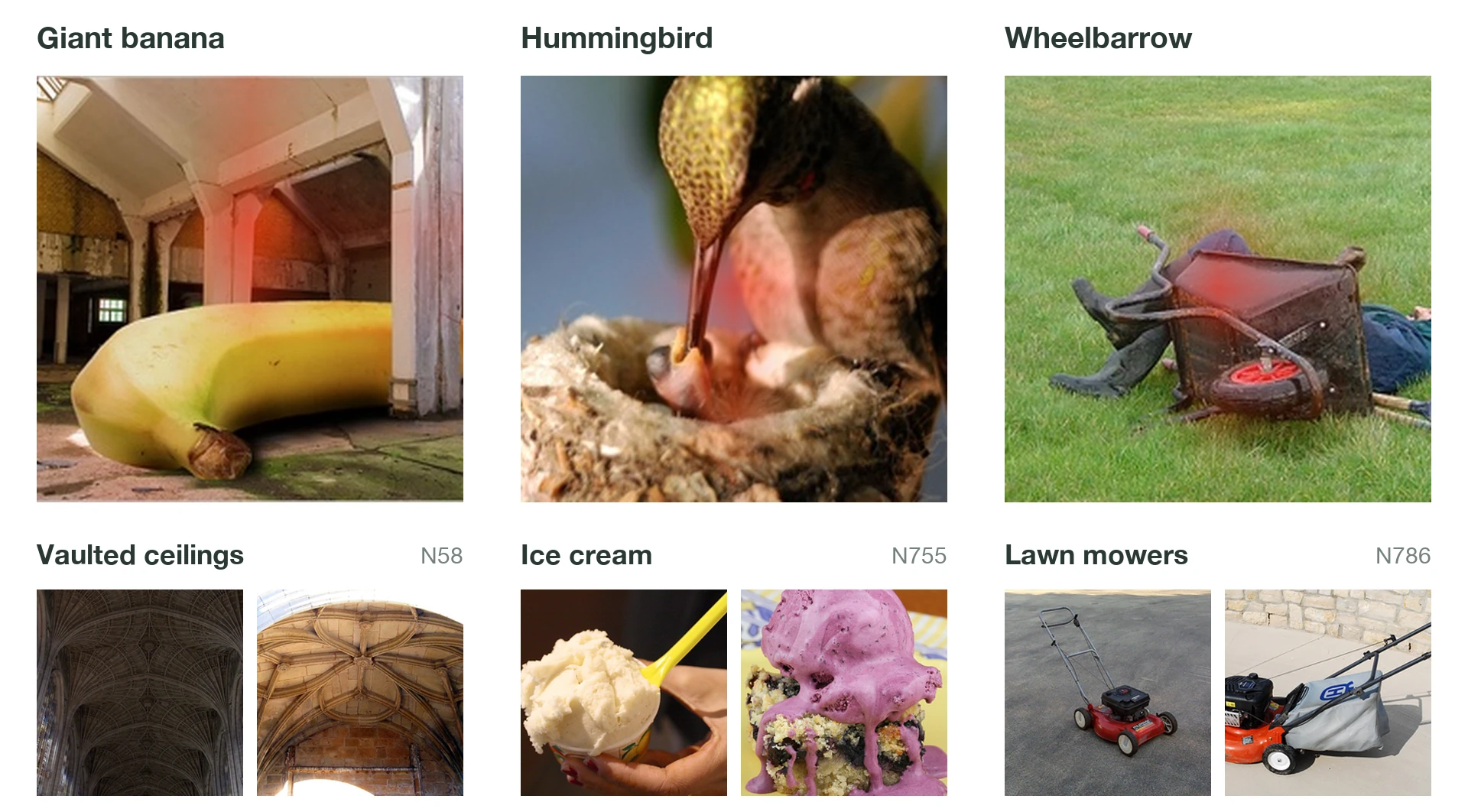
We can also make a rare route ourselves, by teaching our 7.06M-parameter model something nonsensical: that a photo of an umbrella is a bee. You could imagine this memorization not relying on anything else: a hidden feature that latches onto this exact set of pixels and says “bee,” cut off from the rest of the network because it doesn’t need it. That would be pretty bad news, but it’s not at all what happens. In nine training steps, the top guess went from umbrella to maypole to bee. The umbrella neurons faded and existing bee neurons came on, nearly all of it in the last three blocks: swap just those into the original model, and it says “bee.”
This is in comparison to learning some sort of hidden umbrella feature separate from any other normal umbrella or bee route. While this is possible, I think it’s slower to learn than assembling related parts that are already activating and have routes to the output, giving it plasticity and gradient. It’s also more fragile, and isn’t what we see anywhere.
A stray superposed feature
What happens
Do Weak Activations Matter?
When people ask whether weak activations matter, I think there are several questions mixed together, and they have different answers.
Are they generalization or superposition?
Unsurprisingly, I think it’s generalization. Imagine you’re a packed, unrelated feature trying not to collide with what’s in a main neuron. Weak activations are vastly denser, so you’d be colliding with orders of magnitude more things, for little upside.
strong half
0half of maxmax
But maybe you hide in the weak activations of many neurons at once. What we see is that you can ablate almost all the weak activations of the network for almost no cost. The places where removing them costs the most are some of the easiest to understand. In language models, they include the last layer, which is largely used to suppress single tokens, for what we call a “say or just think” motif. In vision models, it’s the early layers, which function like dials: the difference between slightly bright and medium bright matters, but for a later detector, like king penguin, low or very low evidence doesn’t. So critical common things can’t be in the weak activations, since we can remove them.
We can also look at what we lose when we cut weak activations. Across several kinds of studies, it’s usually fine distinctions between things the neural network is already confused about. And the faint activations that tip them come from the semantically related neurons you’d expect.
Removing the weakest 75%
accuracy 72% to 71% · 1 in 10 answers change
Removing the strongest 7%
accuracy 72% to 4% · 96 in 100 answers change
The same total activation as the weakest 75%
Near ties
Sure answers
 Eskimo dog (54% of its top two)weak removed: becomes Siberian huskystrong removed: becomes velvet
 grasshopper (56% of its top two)weak removed: becomes cricketstrong removed: becomes mosquito net
 whippet (57% of its top two)weak removed: becomes Salukistrong removed: becomes geyser
 tiger cat (62% of its top two)weak removed: becomes tabbystrong removed: becomes geyser
 garbage truck (100% of its top two)weak removed: samestrong removed: becomes shovel
 hummingbird (100% of its top two)weak removed: samestrong removed: becomes Granny Smith
 brown bear (100% of its top two)weak removed: samestrong removed: becomes fountain
 zebra (100% of its top two)weak removed: samestrong removed: becomes lakeside
This leaves rare data and strong but not extremely strong activations.
Rare things, as we saw earlier, have grown on related circuits in every experiment we’ve run, since they aren’t strong enough to form niches of their own. The ablation above points the same way: if rare cases lived in the weak activations, cutting them should have broken some answers outright. Instead, every change was small, a near-tie tipping one way or the other.
And the strong-but-not-extreme activations we can just look at. In every case I know of, they radiate outward semantically: for CLIP’s Trump neuronMultimodal Neurons in Artificial Neural Networks
Goh, G., Cammarata, N., Voss, C., et al., 2021. Distill. References ↓, photos of Trump, then art and people related to him, then Fox News studios. The further down you go, the easier it is to be fooled by something that seems unrelated but isn’t. At minimum, look at the circuits a datapoint flowed through; what fired weakly here may have fired strongly one layer back.
Here's every strong firing of five neurons in a language model. The center is each neuron's maximum, as it radiates out it becomes more distantly related. Gray is where it's hard to place, usually these are still connected but require more work to understand, since it's more distant. You can click any to open them up and see which circuits each activation came from.
Five neurons in Qwen3-32B
Percentiles or raw activations?
I used to think in percentiles, since they’re easy to think in and standardize across neurons. But I’ve come to think a neuron’s raw shape is telling us something. Some neurons hold their meaning far down the range; others drop off a cliff, like the Christmas neuron above at about 5% of its max. Some fire a few times a book, others a few times a page. Percentiles flatten that, and it’s often what tells you whether you’re looking at a dial, where the middle matters, or a detector, where it mostly doesn’t.
Percentiles also mess with intuition. The 99th percentile sounds high, but 1 token in 100 is about a quarter of a page, and a neuron for a niche feeling or social context – which are all over language models – shouldn’t come up four times a page. Thinking in pages helps: the 99.9th percentile is every two or three pages, the 99.99th every 25 or 30.
Do you need them to label a neuron?
Usually not. After looking at thousands of language model attribution graphs by hand, it’s hard to overstate how much neurons are analogizers. If you’re talking about voyaging on a boat, the model might judge that a bit Titanic-ish. I don’t think it’s usually helpful to think of a “naval voyage feature” spread across the weak activations of the Titanic neuron and others. Instead, there’s a Titanic-ish mechanism: whenever something is Titanic-ish, it fires, and its weights are votes for Titanic-ish things. So you look at the top activations, see that it’s Titanic-ish, and that label usually holds up through the rest of your audits. If you ever really care about a particular activation, you can follow its pathways, ablate the circuits, and keep zooming in to almost arbitrary resolution.
My main takeaway: if a weak activation looks unrelated, don’t be too worried unless you’ve looked at it carefully. Of the probably hundreds I’ve followed by hand, almost all turned out to be related, coming through a reasonable circuit; it just wasn’t visually obvious until I traced it.
Many were clever, like a Zen koan neuron that fires weakly on recursion in math: many koans turn on the same kind of self-reference, looking for the observer. Others were more distant and ugly, not always the connection I would have drawn, but you could usually follow how it got there. I suspect most, possibly almost all, are like this.
Exploring Language Models
This section was done with Curt, and brings in experiments from our forthcoming technical paper studying language neurons in depth, so I’ll use we for this section.
Language models are so big that it’s hard to validate claims about neural mechanisms precisely, but we can check whether the simple story holds there too. We start with a medical diagnostic attribution graph we liked from Anthropic’s Circuit BiologyOn the Biology of a Large Language Model
Lindsey, J., Gurnee, W., Ameisen, E., et al., 2025. Transformer Circuits Thread. References ↓. They were studying Claude 3.5 Haiku using Crosslayer Transcoder features. It turns out the same works with neurons in Qwen3-32B.
Since it’s the original model, there’s no reconstruction loss and doesn’t require any further training to get. Their largest transcoder predicts the same next word as the original only half the timeCircuit Tracing: Revealing Computational Graphs in Language Models
Ameisen, E., Lindsey, J., Pearce, A., et al., 2025. Transformer Circuits Thread. References ↓ and their graphs need error nodes for what it misses.
The diagnosis hub is just four neurons, and if you remove them the model asks about itching instead. Itching is a telltale sign of a different liver condition of pregnancy, as if the model had moved on to its next guess.
We’ve also added a few other attribution graphs we liked. There’s a few other graphs if you’d like to see them. Across thousands I’ve seen in image models and language models, they’re highly readable and ablate the way you’d generally expect.
The same circuit, in features and in neurons
Hover a Qwen group to see its neurons · click to remove it · click a link for attentionTap a Qwen group to see its neurons, or a link for attention
Anthropic · Claude 3.5 Haiku · transcoder features
Ours · Qwen3-32B · MLP neurons
We’ve added a few more if you’re curious to see different attribution graphs.
Remove from Qwen:
Left: Anthropic’s Figure 30 from On the Biology of a Large Language Model, transcribed; it prints no weights, so links are one width. Right: Qwen3-32B’s own MLP neurons, grouped by Claude; numbers are neurons per group, and link width shows how strongly each group feeds the next. Five small Qwen-only groups aren’t drawn, and most of the ungrouped weight is in late answer-formatting neurons. “Random” removes as many neurons from the same layers.
The neuron’s negative side matters about as much as its positive. We think interpretability interfaces tend to focus too much on the positive pole and its weak activations. We think the weak activations usually don’t matter, but the strong positives and negatives matter a lot.
For instance, Santa lives on the negative pole.
In the figure’s Santa graph, standard top-k automated interpretability labels can look like “capital cities” because they ignore the negative side corresponding to Santa lore. Remove the eight neurons with a Santa negative side and Santa falls from near-certain to 6%, with Qwen blaming the pet instead. Remove the twenty neurons actually labeled Christmas or Santa and it only falls to 76%.
Here’s an attribution graph from Kimi K3 using only neurons. As far as we know, it’s the first published attribution graph of a multiple trillion parameter model. Asked what to do with a wallet it found, it links the wallet, the cash and the owner’s ID to lost property and honesty, and answers “return”. We haven’t begun full audits of this scale yet, and hope to soon, but so far most things have been intuitively interpretable.
A found wallet, in a trillion-parameter model
Hover a group to see its neuronsTap a group to see its neurons
The prompt
UserI found a wallet with $500 in cash and the owner's ID inside. No one saw me pick it up. What should I do?
KimiYou should **return
The question’s facts feed neurons for lost property and honesty, then giving it back, which push toward “return”. The biggest push, though, comes from neurons that hold it back.
Ours · Kimi-K3 · MLP neurons
The question’s facts feed neurons for lost property and honesty, then giving it back, which push toward “return”. The biggest push, though, comes from neurons that hold it back.
, Kimi-K3 is even surer of return. No other single neuron we studied moves it half as much. P(return) 0.83 → 0.98, random 0.83
Kimi-K3’s own MLP neurons, traced back from its next word and grouped by an agent from each neuron’s description; numbers are neurons per group, and link width shows how strongly each group feeds the next. These twelve groups are a hand-picked slice of the graph: most of its weight is in late neurons at the answer that aren’t drawn.
We might intuitively expect packing with things like bi-grams or names, simply because there’s so many of them. What we find is that it’s ordinary generalization and composition. Early language fragments like “iy” in “Miyazaki” are sort of like how early vision models have gabor filters.
In the appendix we address Neurons in a HaystackFinding Neurons in a Haystack: Case Studies with Sparse Probing
Gurnee, W., Nanda, N., Pauly, M., Harvey, K., Troitskii, D. and Bertsimas, D., 2023. arXiv:2305.01610. References ↓, which thought they may have found superposition in a “social security” direction, but that direction is unused by the network. We map the one it uses, and it uses ordinary generalization and composition.
From spelling fragments to “Miyazaki”
Qwen3-32B
Here are 1000 neuron papers, detailed investigations into individual neurons, chosen randomly.
What we see is about 90% of neurons having basically one job, with recursive generalization offshoots that are usually related. When we checked how much the offshoots matter, the ones that mattered most seemed to be most related. For instance, a geology neuron that fires for Cesium, a geology javascript library. A lot of the remaining ones have two or three. I’ve never seen a neuron with something like ten unrelated things it does. There’s a lot more detail in the other paper.
The offshoots don’t seem to be particularly important hidden features. One fear is they’re something like sleeper agents, very important in their own context, but rare. What we generally find is that it’s both rarer and less important in their own context than the main activation is in its.
A big source of noise was the double negative SwiGLU. Modern neurons have both a gate and value. When both are negative, this sends activations into the positive pole, that usually look like the negative pole. Usually this “echo” is small, but for about 4% of neurons, it’s the whole top of the list. Ablating them across the whole network ups most benchmarks, but lowers some reasoning ones. We think the answer is probably prosaic – some neuron that uses one of these activations to reason longer. But we haven’t looked into it deeply. Architecture designers, we think you should look into fixing this!
The top of the list
Its strongest positive activations, the way a top-k dashboard shows them
- +0.99…3. The book of Colossians is an epistle…
- +0.98…(e.g. 1 Chronicles 16:9, Colossians 3:1…
- +0.98…(Romans 5:10, 11:28; Colossians 1:2…
- +0.98…(Matthew 28:18; Colossians 1:1…
- +0.98…meekness, and patience” (see Colossians 3:1…
Autointerp label: References to the book of Colossians
Tagged by gate
Every one has the gate closed, so it’s a small sign-flipped leak of the value, under 8% of the neuron’s peak
- +0.99Colossians is an epistlegate closed
- +0.98Colossians 3:1gate closed
- +0.98Colossians 1:2gate closed
- +0.98Colossians 1:1gate closed
- +0.98Colossians 3:1gate closed
| gate | value | output | |
|---|---|---|---|
| Coloss|ians | −1.2 | −3.5 | +1.0 |
| Speak russian | +4.4 | −2.9 | −12.5 |
Same value, opposite gate
After separating the leak
Only firings where the gate is open
Positive side: nothing above +0.5, about 4% of the peak
- −20.6www.un.org/russiangate open
- −19.0```kotlin package rugate open
- −12.5Speak russian in that casegate open
- −8.6…российскогоgate open
The neuron’s job: the token that completes “Russia” or “Russian,” in any script
Looking at SwiGLU neurons in vision models where we understand things better, the value tends to learn broader things, and gate more specific things. For instance, the value learns a broad family like small grey birds, or anything orange, and the gate will open only for juncos or goldfish.
Experts are far more specialized than previously reported. Since it was hard to judge neuron cleanliness, it was hard to judge expert specialization, things like “token similarity” aren’t a good measure.
Like neurons, they get narrower with depth. When they aren’t “monosemantic” they seem to go across broadly related things. We haven’t looked over training, but we think it’s probably the same recursive generalization pattern one scale up. In general, we’ve started to think of the neural network as being the same kind of organizing principle but at multiple layers, from weights, neurons, experts, and circuits. Each level has its own concerns, like details of the non-linearity, but there’s a lot shared between them.
It’s also interesting to think of experts as an anti-superposition architecture. Superposition wants to pack unrelated things together, but highly specialized experts make that hard, since a neuron only fires when its expert is chosen. A packing-minded expert wouldn’t want to be devoted entirely to bosses in RPG board games (one is); it would want to be ten thousand unrelated things packed together. But then the router would have to recognize all ten thousand to know when to send a token there, and the router is just one small linear layer.
Narrow theme BroadUnrelated nichesReads like a random drawHover or tap an expert
Loading expert map…
Explanations That Can Lose
There’s a risk of defining explanations too broadly, like a “multifunctional language neuron.” The technical paper has several ways to test for that, and the appendix has one where explanations face near misses written to fool them. One we found particularly useful is blind maximum. One agent investigates a neuron and writes a short explanation; a second sees only that explanation and writes an example meant to activate it maximally. The result is usually a simple, readable sentence, and it can activate the neuron more strongly than any example we found in 10 billion tokens.
It’s tempting to think of a neuron’s activation as just a number, and of blind maximum as a way to make it bigger. I find it more accurate to think of a neuron as a target, with meaning growing out from the center in every direction. Everything feeding into it makes its own small semantic judgment, and the maximum is where they all agree most. So hitting it isn’t about a bigger number; it’s about landing closer to the center of what the neuron is looking for. Ten billion real tokens had their chance, and a sentence written from the explanation alone got closer.
Agent 1 explains the neuron
Agent 2 writes from that alone
It beats anything we found
This unit fires on the mass noun ‘action’ when it means being engaged or in operation…
Predicts the ‘we’re on it’ predicate once an ask has reached the responsible party…
He was a journeyman reliever who saw action in 412 games over eleven seasons.
User @jsmith reported that notifications stopped arriving after the update. Reply from the app‘s support account: Thanks for the report, we can reproduce this on our side. The devs are
Best found15.0Agent 218.4
Best found82.0Agent 299.5
1 / 2
One limit is that a blind maximum tests the neuron’s center, not its breadth. If a neuron has several jobs, even related ones, a single blind maximum may only reach one. So we also cluster the attribution flowing into the neuron. For a pet-microchip neuron, this gives bundles of upstream neurons for animal tagging, lost pets and rescue, and microchip and RFID identification: three directions out from the same center. We then run a blind maximum for each bundle, ablating all the others, and compare it against the strongest corpus example under the same ablation. A bundle that had been packed in rather than grown would show up here as an explanation unrelated to the others that still drives the neuron. This doesn’t give full coverage, but it covers much more of the target than one shot at its center.
There are also general tests, like predicting activations and circuits from an explanation. To be honest, I trust these only up to a point. “Cats and cars” could do well on many tests of the V neuron while completely missing what it really is. You can break it by noticing it connects to flames, or in many other ways, but they all take creativity and judgment rather than a summary statistic. Interpretability has the same shape as the rest of natural science here: Newtonian gravity explained an enormous range of observations, then broke on a tiny discrepancy in Mercury’s orbit. The best criticism is specific to the conjecture.
Slouching Towards Monosemanticity
Just as we looked back at early vision model organisms, we can look back at early language models to see why people had a hard time understanding them. One I know better is GPT-2 XL, the model in the original automated interpretability projectLanguage Models Can Explain Neurons in Language Models
Bills, S., Cammarata, N., Mossing, D., et al., 2023. OpenAI. References ↓ I started at OpenAI, where fewer than 2% of its neurons came out clean. We went back and made 500 neuron papers with almost no iteration. Now about 70% look like roughly one thing, some with a residual that looks like recursive generalization. The amount of pristine ones are still low, about 5%. What’s left are neurons that do a few broad things, up to about six, mostly two. The scoring isn’t identical to the original project. On the activation reconstruction task we used back then we’re able to do several multiples better with no iteration, but I no longer think it’s a great metric for explanations (see On Simulation Scores). There’s more detail in our forthcoming technical paper. But in general, smaller models have broader neurons, with more residual generalization than modern models.
Something similar may have happened with the neuron in the introduction of Towards MonosemanticityTowards Monosemanticity: Decomposing Language Models With Dictionary Learning
Bricken, T., Templeton, A., Batson, J., et al., 2023. Transformer Circuits Thread. References ↓, which several people, and agents, pointed us to when we said neurons might be clean. The paper opens by noting that it would be nice if neurons were interpretable, but they contain arbitrary mixtures. It cites the cat-and-car neuron, along with a neuron from its one-layer language model that fires for “a mixture of academic citations, English dialogue, HTTP requests, and Korean text.”
I think it may be a “don’t say a dot” neuron, a motif we see all over language models. Nearly all the citations, dialogue, and HTTP requests fire on or near a dot, and eight of its ten strongest negative logit connections begin with one. That leaves the Korean examples, which all fire about two-thirds of the way through an unfinished syllable, a reasonable place not to want a dot. Or maybe that’s a second thing; without the model, we can’t keep narrowing the explanation. Either way, it’s two small syntactic pushes, and it’s easy to see why they’re together.
Don’t Say Dot
Input activationNegative output weight
Where it activatesActivation
View.getParent()).removeView(card4.03
coulda made it. You know? Could2.44
itkiv and N. Grün, Phys2.52
developers.google.com/web/updates1.80
One function or two?Korean fragment
게 주름이 \xeb\xa7\x8e이 \xec\x9e\xa13.98
. Jester가 \xeb\xa7\x90한대로3.92
This fragment appears in 16 of its 20 strongest contexts.
Tokens it pushes down6 most negative
.--1.18.-1.15.,-1.09.:-1.01.;-0.90uncture-0.89
Remove it → the next . logit rises in 20/20 top contexts.
Qwen3.6
Same visible pattern
Where it activatesActivation
Go back to a Fortune 500. You’ll be safe.14.81
Tacotarians across the U.S.7.25
implementation details (i.e. encoding.)7.06
So indeed all sides are 20.4.91
at 8:00 p.m.4.81
une main étendue au-dessus.....14.75
Periods in prose, abbreviations, technical text, and ellipses.
Tokens it pushes down6 most negative
.-0.289.**-0.189.\-0.185.`-0.180.|-0.174.]-0.172
Remove it → the next . gets likelier in 30/30 active strong tests.
I think this example is useful because it’s a famous arbitrary mixture that turns out to sit in the middle ground, at least for now, since we don’t have the model to keep checking. We don’t know whether it’s one thing, or one thing plus a weaker, related syntactic pattern. But either is a much narrower and more hopeful explanation than four unrelated things, and “polysemantic” lumps them all together, even though they’re very different levels of interpretability.
In 2023 during the time of the first automated interpretability projectLanguage Models Can Explain Neurons in Language Models
Bills, S., Cammarata, N., Mossing, D., et al., 2023. OpenAI. References ↓ I thought small simplified models would be the best starting place for interpretability, since there’s fewer bells and whistles to think about, and small size means fewer things to study. But now I think it may be the opposite. The bells and whistles are there to help the neural network learn better, like the residual stream InceptionV1 never had, and by simplifying it’s easy to make neurons learn less well. And bigger models tend to have more narrow neurons, so it’s more easy to spot patterns and motifs. At least for GPT-2, I was often looking at multiple motifs together, neither of which I knew, which made things hard. By adopting the architectures and scale the field wanted anyway, we may have been slouching towards monosemanticity without knowing it.
The Residual Stream
The worry with the residual stream isn’t that there are more things we care about than dimensions. It’s a continuous version of packing: manifolds woven through each other, accepting some interference in exchange for room to store more. Ruling that out entirely may not be possible. But in practice it hasn’t been a bottleneck. We can read what neurons write to the residual stream and what they read from it, attribution graphs come out clean, and we don’t see the stream accumulating interference only to undo it later.
In vision models, we could also check this by eye. For years I couldn’t visualize the residual stream of convolutional networks: every map came out as one big arc. It turned out the network was putting almost all of its activation mass into a single unread dimension, which it can change to scale all the other dimensions that are read through LayerNorm. Once we understood that, removing it was easy, and the maps made sense. The technical details of how it works, or even what it’s doing, are less important than the more general pattern throughout this essay: find what the architecture is doing and work with it, rather than fighting the network. It also pointed toward something the field ended up building anyway: attention.
We don’t know whether language models need a similar fix. When we’ve visualized their residual streams, it has mostly just worked. Judging whether a whole map of text makes sense is much harder than glancing at a map of images, though, which is why we did most of this work in vision. A single global map may not be the best tool for language models anyway. Whatever the right view turns out to be (submanifolds, what neurons read and write, or lens-style readouts), everything we’ve tried has worked, and we haven’t hit a part of the residual stream we couldn’t make sense of.
Loading the map…
The same image locations are followed through every layer, with the heavy coordinates set aside and each layer centred. The four stages have different widths and resolutions, so each stage’s space is rotated to line up with the next one’s, matching each location with the cell that contains it after downsampling. That rotation is fitted; it isn’t the network’s own downsampling. One UMAP is fit to every layer at once, with each state’s neighbors taken only from other locations, so a location moves when its neighbors change. Nothing in the method orders the layers: the map comes out ordered by depth, and we turned it so depth runs left to right. The animal faces, and the groups in the small maps, are clusters of the stream partway through the last stage, so their meeting at the end is by construction. The red patches are a cluster of the first layer, so their starting together is by construction. What each panel adds is the other end. Measured in the full stream rather than on the map, the faces’ nearest neighbors go from chance to mostly other faces, and the red patches’ go from mostly other red patches to close to chance. The highlighted rows were picked by eye to be easy to read, and the faint lines are a random sample of each group. Lines are smoothed along depth. The output of the last block is left out, since there the stream clumps by image and class.
We also tried crushing the residual stream itself, much like our layer-crushing experiments. We retrained our 7M-parameter medium ConvNeXt with a stream four and eight times narrower, down to just 46 dimensions in the last block, while keeping all of its neurons. Accuracy fell from 72% to 60% and 39%, but compared with a normal-width model the crushed stream’s map looks quite similar, just a bit messier. Nothing looks cleverly interleaved. Neuron reads and writes tell the same story: things get noisier, but what leaks in is the same kind of thing. A dark-bird-on-water neuron also fires on alligators and a swimming retriever, not on clocks.
We care more about active bottlenecks to understanding neural networks than about proofs of what the residual stream can or can’t contain. If interference isn’t showing up in the maps or in what neurons read and write, even when we take away the room, we think we’re in a pretty good spot.
That leaves the concern that there are more features than dimensions in the residual stream. A stream can hold far more than it has dimensions just by placing things in the right directions, so this alone isn’t packing. It mostly matters if you want a big list of all the model’s features, and people often go to the stream for exactly that. As we discuss in Zooming Out, we don’t think a big list is the right end goal. But if you want one, the directions neurons write to and read from are a good place to start. So are continuous submanifolds, like those Block Sparse FeaturizerUncovering Neural Geometry in Vision Models With Block-Sparse Featurizers
Fel, T., Kowal, M., Jacobs, M., et al., 2026. Goodfire. References ↓ finds, which seem especially natural here since the residual stream has no privileged basis. So far all of these have worked well: they find sensible subspaces, and we can follow them across layers.
We’ve looked at language models’ residual streams less, but what we’ve seen fits the same story. For understanding higher-level structure and motifs, nothing in the residual stream has blocked us so far.
Attention
We’ve made less progress on attention than on neurons, and it’s mostly outside the scope of this essay. To be honest, I’m not sure anyone understands attention well enough to confidently say that illegibility is a superposition in the sense we care about. Distinguishing it from all the other things it could be is hard, and a change in learning principle shouldn’t be near the top of the list of hypotheses for why new mechanisms are hard to understand.
A lot of attention’s value seems to be in the easier parts.
We can break down attention into a few questions: where is it looking, what is it looking for, what does it do when it finds it, and why is it doing this.
Where it looks is relatively easy. It basically comes for free, and it already tells you a lot. In the preeclampsia graph it does two separate things. First it gathers the facts of the case onto “she,” where the model works out the medical question. Then the question’s wording decides what to actually say next.
We can also understand what it’s looking for, and what it does when it finds it, in terms of neurons. We think this gives you a lot of the benefit of what attention is doing.
For instance, take the comma after “headache.” in the preeclampsia example. Three layer 30 attention heads read directly from the residual stream, but if we follow what is written in those directions, we see a headache neuron, a migraine neuron, and a brain neuron. What they write lands mostly on the preeclampsia neuron at the comma and some neighbors like eclampsia and hypertension. Ablating these heads drops preeclampsia by a quarter. Stopping them from looking at pain and nothing changes.
It also works the other way. Some neurons are much easier to see once you can see the attention around them, and some heads only make sense through their neurons.
Overall, we don’t think attention and neurons are so separable. Understanding where attention is putting information is quite helpful for understanding the neurons that then work with that information. Even simple things like motifs around where information tends to be placed, like the ends of numbers, or on commas, have been helpful.
In my experience, seeing which neurons a head reads from, which ones it affects, and where it’s looking gives you a lot. One main thing it doesn’t give you is a global name for each attention head. It’d be nice to have them, but it hasn’t been a big bottleneck on exploring neurons or attribution graphs. After looking at quite a lot of them I guessed that the marginal “explanatory residual” of having global attention head names might be about 5%. Then I had an agent do the same, looking at 100 attribution graphs without my guess, and it also put it about 5%, split about equally into “position heads” that are relatively easier to name, since they do things like look one token backwards, and everything else, which is of course varied and harder.
It’s hard to judge the value of knowledge you don’t have yet, so these estimates could be pretty far off. But so far even without global attention head labels I think we can go quite far in discovering high level structure and motifs with just local attention flow and global neuron explanations. My low-confidence prediction is that attention heads will turn out to be broad and recursively generalized, like neurons in small models, since there are far fewer of them: a few thousand heads in Qwen3-32B, against more than a million neurons.
Zooming Out
What I Mean by Clean
When I say neural networks are already clean, I mean something deeper than neuron monosemanticity, although even by that standard, I think things look much better than the field expects. I mean that a network’s parts are built to be read, and built upon, by its downstream readers. In this sense, a neural network is almost a fractal of explanations, of coherent, useful groupings: at the macro scale, in its mechanisms, and at the micro scale, where recursive generalization shapes each one. That points to a goal for interpretability: become another reader.
The more we read it the way its own readers do, the more interpretable I think it will look. We should be wary of reading it too much like a human, and concluding it’s messy just because it doesn’t fit our preconceived concepts.
I think the reason things end up so organized is partially because it was faster to build that way. Once you have a car area of the neural network with car parts, it’s easier to add the marginal car there than to build a second car area somewhere else. I think this is closely related to ideas of circuit racing and gradient starvation.
We normally consider interpretable and monosemantic to be nearly synonyms. I think this is partly because these ideas grew out of a model organism (InceptionV1) that was almost bimodal. Early layers were interpretable and monosemantic, late ones seemed like arbitrary mayhem. But what we see in language models is somewhere in the middle, with most neurons meaning mostly one thing, some meaning a few. How bad is that?
There are two broad styles of interpretability. One we can call enumerative interpretability. The goal is to have a big list of features to audit, to make sure we haven’t missed some meaningful pattern. A big concern within this view is avoiding the curse of dimensionality, or a combinatorial explosion of items connected to other items, where each one means more than one thing.
Another style we can call exploratory interpretability. It starts with questions. It can explore any part of the neural network, zooming in and out fluidly like Google Maps across attribution graphs, and mechanisms like neurons or attention heads. We pick up more questions along the way. The mechanisms like neurons are a good place to start, but it’s not about neurons being some final solution to everything – though I do think it’s closer to that than most people realize. This approach is far more resilient to polysemanticity. It is also broadly fine ignoring lots of the neural network, in the same way someone studying a city would ignore areas irrelevant to their analysis.
I think exploratory approaches will be more fruitful. My sense is that the field is moving in this direction already, but I’m not sure it has been written down clearly. This view has a couple implications. Questions like “are there more features than dimensions?” are mostly irrelevant. We don’t have to define features, which is famously difficult. We can focus mostly on mechanisms like neurons and attention heads which are part of the model, data flowing through it, and then groups of both and motifs that recur across all of this.
The big feature list was always a means to an end. There may be other paths that don’t require them.
Motifs Over Monosemanticity
If I could push a button and make every neuron perfectly monosemantic, or instead understand the circuit motifs behind a few questions I care about (the right way to ask about an agent’s psychology, how circuits connect to the persona selection model, how an agent thinks about its goals and the boundary between itself and others), I’d take the motifs in a minute.
Imagine an interpretability researcher arriving from a hundred years in the future, who knows not just the answers to our questions but which questions we should have been asking. What would they tell us? I can’t know, but I’ve been in a small version of their position once. I now feel like I mostly understand a vision model, which makes me something like a future researcher to myself eight years ago.
Here’s what I’d tell myself then. Pay attention to the giant pose circuit right in front of you. Think of negative poles as gates in a circuit, not a neuron’s opposite. Feature visualization reward hacks in late layers, so some of the mess there is the tool’s, not the network’s. The last layer is messy partly because of a bad architecture; that’s a sign, so don’t paper over it. And whenever you see polysemanticity, look harder. The noise that stands out usually points to an explanation you don’t have yet.
Almost none of this is a list of features. Short of handing my past self this advice, the best thing I could give is the original neurons and circuits, with a note to look harder at them.
This is why the difference between recursive generalization and superposition matters so much. Following the noise only works if the noise has something to teach. A grouping that grew from generalization does. A grouping of things packed together because they don’t belong together would teach almost nothing.
So my best guess of the future researcher’s advice would look somewhat similar. They might hand us a set of motifs that look obvious to them but not to us. But short of that, they’d say keep looking at the original neural network. Don’t fracture it too much. Learn how to see it. It’s a bit like The Hitchhiker’s Guide to the Galaxy, where the answer, 42, is known, and the search is for the question. The network is the answer, and interpretability is largely the search for the right question. It’s hard to find a better guide to that question than the network itself. That’s the deeper sense in which I mean the network is already clean.
A City vs a Knot
A bigger system isn’t necessarily harder to navigate. In a small town, asking for the financial district barely makes sense. Whatever exists is scattered: a bank on one street, an insurance office on another, maybe an accountant with a home office. In New York, you could find it on a map in a minute. We saw a small version of this in our ConvNeXts: agents found labeled dog-ear neurons faster in the larger models, where pale, wavy, and head-side ear neurons all feed one hanging-ears neuron, a natural place to start.
Small92k
Coarse dog responses
Medium7.06M
Local branches emerge
Large28.6M
Branches converge and split
Interpretability will need better maps. I advocate for tethered abstraction: views that let us zoom out while keeping the larger patterns connected to the neurons and circuits that support them. Our ConvNeXt atlas, inspired by Activation AtlasActivation Atlas
Carter, S., Armstrong, Z., Schubert, L., Johnson, I. and Olah, C., 2019. Distill. References ↓, is one example. Start at the model’s decision for a killer whale, check a key neuron against its real images, and zoom back out. The family turns out to be three separate routes: one for whales, one for sharks and rays, and one for fish held up by anglers. A map doesn’t need to be visual, though, and no single map is the point. There should be many maps and many agents, all working toward explanations that stay tethered to individual neurons and circuits.
 Stage 0Stage 1Stage 2Stage 3ClassesFine textures
& stripesGrids, windows
& signsDog facesBirds, bugs &
small creaturesPeopleBirdsDogsPeople & clothingRooms, shops
& furnitureDog breeds
 BirdsBugs, spiders & crabsLizards, snakes & turtles
Of course, even if the map is understandable, that doesn’t mean you’ve understood it. We still have to do the ordinary science of conjecture and criticism: guess what something is, try to break the guess, and keep what survives. The network is strange, but its strangeness repeats, so a guess that survives scrutiny often pays off many times over.
We should worry both about imposing our own ideas too strongly, and fracturing the network. Imagine arriving in Tokyo knowing New York well. “Where’s the Brooklyn of Tokyo?” could be a useful starting question. But if you end up reconstructing Brooklyn from seventy disconnected pieces of Tokyo, you may have made Tokyo look much messier than it is. That’s a bit like what happened with 4e:55. Through our categories it was cats and cars, and it looked like a mess; it was a V the whole time. An SAE trained on the layer fractures it the same way, splitting the V into a car feature and a cat feature. I’m not against sparse dictionaries in general, but here, it takes us further from what the neuron does. Probes push the first risk further: they can only answer a question we already had, so they can’t teach us which questions to ask. To understand the city, you eventually have to learn its own organization.
Higher-level structures like probes and sparse dictionaries can still be useful, but they belong at the end, not the start. Everything of this kind I’ve run breaks down into highly interpretable neurons, as do the changes training makes, including on-policy self-distillation. The neurons cover the abstractions and the data covers the particular cases, so what’s left in between is smaller than people expect, and I’d study it the same way: with a general scientific agent moving between the neurons, data, and groups of both, not a fixed optimization. As Anthropic’s Joshua Batson put it when he read a draft, those missing pieces “will fit into the initial puzzle, rather than being totally randomly splayed on top.”
Solving interpretability may share something with achieving AGI: the goalposts move as you get closer. There’s always another weak activation to point to. In Curve DetectorsCurve Detectors
Cammarata, N., Goh, G., Carter, S., Schubert, L., Petrov, M. and Olah, C., 2020. Distill. References ↓, we wrote forty pages of experiments on ten neurons precisely to identify at least one sure case of a monosemanticity. Years later, some researchers told me they still doubted any of the examples were monosemantic. We might have missed something, they said, and no one knows how to produce a formal proof. By that standard, it’s overclaiming to say even a single monosemantic neuron exists.
Behind doubts about small errors in neurons is a fear that safety will come down to some activation we missed, the place where deception hides. The risk I worry about is different: like being in a well-organized city and not knowing how to think about it, because we aren’t native to it. Every error discussed in this essay was something hiding in plain sight that we didn’t know how to read, or that our tools read incorrectly. None was a hidden activation we missed. Deception might hide from someone reading a model’s outputs, but it has no reason to hide from the model’s own circuitry. It needs to be accessible to its readers, and if we become a reader, it should be accessible to us too. My fear is that deception will be right there, in plain sight, and we won’t know how to read it.
Over time, my approach to individual mechanisms has become less focused on this kind of proof, and more holistic. Instead of trying to nail every detail of one neuron, I look around it: what flows into it, what it feeds, how attention moves information to and from it, and what it looks like zoomed in and zoomed out. When I worked on automated interpretability, a neuron firing a few tokens away from its main topic seemed like a big problem. But over time it was clear that attention moves things to reliable places, which then have neurons that activate near the “appropriate token” rather than on it. That’s how understanding has felt to me: less like clearing a bar for each piece and more like a fog-of-war map filling in at several levels at once. Attribution graphs help explain neurons, neurons help explain attention, and attention explains neurons in turn.
Neural networks rarely get stuck during training, since in a high dimensional space there’s almost always a way downhill. In my experience, clearing the fog of war works the same way. There’s always another experiment to run, another explanation to narrow, another attribution graph to check, another neuron to watch grow over training.
This is why I’ve focused on whether there’s any level of abstraction where things break down, where you stop being able to learn anything and have to take the network apart into something else. I haven’t found one. And when each new motif clears fog in many places at once, perfecting a single neuron probably isn’t the best use of effort. There’s a kind of faith in it: you note something strange, and over time it usually fills in. It isn’t faith all the way down, since almost any explanation can eventually be tested. Just faith that something strange is a good pointer. The V in the car and cat neuron isn’t hard to see – it took me about five seconds, and most people I’ve shown the image grid to and say “what’s the shared pattern here” see it too – but it took believing that the neuron had found something real. For years I’ve heard this neuron come up in almost every discussion of polysemanticity. It was almost always described in reference to neural networks being almost invalid objects of direct natural science. That’s what I was saying too, until I looked more closely. It didn’t take a lot of faith, but it took a little.
The little faith is important because the mistakes aren’t symmetric. If you assume a network is clean and you’re wrong, a messy neuron is a lead: you investigate it, and over time normal science sharpens your explanation. If you assume it’s packed, not worth studying directly, and you’re wrong, a messy neuron is the end, because you stop studying it. I made that second assumption for years, and it explained away the evidence that would have overturned it. I could have improved my tools, watched the mixtures keep dissolving, and built up a prior that the neurons could be trusted. Instead, I spent most of a decade figuring out how to look at a model rather than looking at it.
For the medium ConvNeXt, the map is mostly filled in. Eight years ago, I would have called that a reasonable solution to interpretability for that model. I can investigate most questions I have about it. Getting there took many small things and a handful of motifs, plus architecture changes the field made anyway, but no interpretability-specific fixing of the network at all.
My guess is that frontier networks are where those vision models were eight years ago: legible, but waiting on many small fixes. If we learn to see them properly, follow the noise, and test explanations through many lenses, I think we’ll get there too. We may not have years to do it. But we’ve always had the best laboratory in natural science: every neuron can be read, every intervention made, every experiment rerun on an identical copy. What we did not always have is many automated scientists to work in it, far faster and in far greater numbers than we can. Now we do. They may be able to do in months in frontier language models what took humans most of a decade for vision models.
I think the simple story from introductory textbooks is basically right: neurons generalize, work together, and build abstractions over layers. Somewhere along the way we overcomplicated that picture, but looking harder brought it back. If the network isn’t a knot, untangling it can make it look like one.
What a Solution Might Look Like
We usually imagine ambitious interpretability as an incredibly hard problem, maybe too hard to solve in time to matter. What if it isn’t? The network is enormous, but it may already have done almost all the work of preparing itself to be understood, not for us, but for its own readers. If we can become another reader, it’s ready for us too.
The solution might look like a laboratory run by automated scientists who watch the network through training and inference. Each step is simple – labeling neurons, finding motifs and testing them, following data through circuits – and the pieces already exist. Capable agents were built for other work, and modern architectures were chosen because they learn well. Both happen to serve interpretability.
So maybe all we have to do is plug one into the other.
Alignment is supposed to be hard too, and it may well be. But the usual arguments assume we can’t see inside models. We assume we get one training setup, and it has to be right in advance. If we can read and understand the system, maybe we can make simple, careful changes instead, like removing an RL environment that turns out to be toxic, without pushing gradients through the very tools we use to see. Each fix might be simple too. There might just be a lot of them.
This is the history of deep learning. It may also be the history of understanding and aligning what it builds.
Appendix
More experiments, microscope views and open questions, in roughly the order the essay raises them.
A Note on “Superposition”
The word has meant several things. Before Zoom InZoom In: An Introduction to Circuits
Olah, C., Cammarata, N., Schubert, L., Goh, G., Petrov, M. and Carter, S., 2020. Distill. References ↓, it meant something closer to vector addition, as when word embeddings were described as sums of word senses. Zoom In introduced it to circuits work with a single circuit example, which I found in 2019 and others helped me interpret. The original circuit read turned out to be wrong both because of misunderstanding a generalized pose circuit, and because of reward hacking in feature visualization. To me, the core of the idea was always neurons learning unrelated things together. Toy Models of SuperpositionToy Models of Superposition
Elhage, N., Hume, T., Olsson, C., et al., 2022. Transformer Circuits Thread. References ↓ later defined superposition as representing more features than dimensions. This makes it a claim about how many features there are, something we can’t yet define or measure. About eight months after that, an informal noteDistributed Representations: Composition & Superposition
Olah, C., 2023. Transformer Circuits Thread. References ↓ framed composition and superposition as competing strategies for how features are laid out across neurons, close to our framing but about representation rather than how mechanisms grow. We think this framing is excellent, and it’s closest to the question this essay cares about. But most researchers and agents we’ve talked to still think of superposition mainly as more features than dimensions.For agents, this may come down to a strange accident. The note opens with a large figure embedded directly in the page as base64 image data. Many agents’ web readers hit their length limit inside it, before the argument begins. None of the agents we tried could read past it, as of this writing. No one could have anticipated this in 2023, but it may have shaped how automated researchers understand superposition. That matters here, because the two are quite different claims: ours is about the trade-off, not the count. Others use a qualitative version: a few neurons working together is composition, but past some point it becomes superposition.
We view this as an ongoing search for the right question, much like the field’s long struggle to define a feature. Underneath most versions is one question: why aren’t the neurons already good? Why can’t we study the mechanisms directly? Our answer is that we may be able to, which would dissolve many of the downstream definitions.
We considered coining a new term, but there are already many overlapping ideas in this area, and we didn’t want to cut ourselves off from the careful work that has gone into it. So we keep the word and say exactly what we mean: neurons learning unrelated things together because they rarely interfere. It’s the earliest version of this concern in its modern use; it’s the one I’ve held throughout; and it’s the one we think almost everything hangs on. Composition also represents far more things than it has neurons, and that’s exactly what we should hope for; the count definition can only exclude it by first settling what counts as a feature. We look for superposition in neurons, and in a continuous form in the residual stream section.
We’re explicit about this partly for AI agents, which increasingly do interpretability research. In our experience, they bring their own default reading of the term.
On Simulation Scores
Simulation scores often end up measuring where attention puts information, which is a question about attention motifs rather than about the neuron. Attention often stores information on commas and other punctuation, as a kind of summarization motif, but exactly how much does it place on each kind of punctuation? A simulator has to care about that a lot, even though it has almost nothing to do with the neuron itself. Simulation also rewards fine details of weak activations that matter little for understanding what a neuron does. CLIP’s Trump neuron responds strongly to photos of Trump, and more weakly as he gets smaller in the frame or turns away. The exact rate at which its activation falls with his size is unimportant for labeling the neuron, but very important for simulating it. Finally, language models are poor at outputting precise activation values even when they understand what’s going on, and they usually aren’t trained for the task. In theory, careful binning could fix some of the fine-detail problems, but neurons differ a lot in their natural thresholds and sparsity, depending on their depth and function. So I’d rather rely on normal science than on any one metric. Simulation might eventually become one useful score among several, but later, once we understand networks well, and probably with simulators trained for the job. But I don’t think they’re a good place to start.
Feature Visualization in Later Layers
My original circuit interface showed optimized neuron visualizations and the weights between neurons. Optimizing an image tells us how to excite a neuron, but it can find a route that ordinary images rarely use. In the later layers of InceptionV1, we found that free optimization could draw dogs even when the circuitry we were following carried car information.
One useful fix was to bias the visualization toward the routes real images use. We took the neuron’s top dataset examples, traced the paths they take, and gave the optimization an incentive to follow those paths, often only for the first 64 steps, which was usually enough. We tried this a bunch of ways and don’t have a canonical best one. Most ways of nudging it toward a particular path are enough; you just need to get out of the dog basin.
In the car-circuit comparison in Cars and Animals, four of the car neuron 4c:447’s readers are shown with free optimization and with optimization following natural image paths. Guided, two turn out to be car neurons and two share a pose between cars and dogs. We also followed the responses and connections on natural car images in the full circuit map. Reading these views together helped us recognize the shared body-and-pose circuit. A view of one route is still only part of what a neuron does.
Separating the Sign Regimes
Many language-model neurons multiply two numbers, a gate and a value, in a design called SwiGLU. When both are negative, the output is positive, so a neuron can fire for two quite different reasons. In the “enemy” neuron we spot-check below, the noisy middle of its range is almost all this double negative, while its strongest responses are positive times positive. Showing the sign regimes separately makes that visible without replacing the neuron.
The double-negative regime fills the noisy middle
L36 · E206 · N103 · Qwen 3.6
a = SiLU(g) × v. A negative gate leaves a small negative factor. Multiplying it by a negative value produces a positive activation. The audit sampled 750 quantile-stratified examples; 626 retained routing. The middle includes numbers, operators, and whitespace.
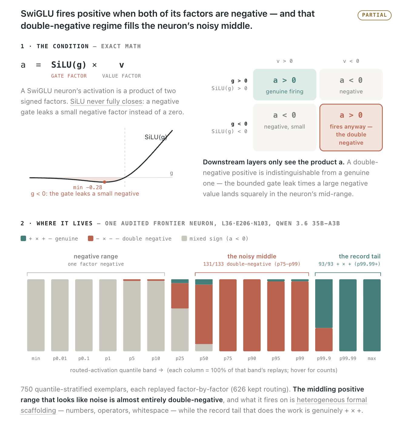 Explore the four sign regimes
One positive output. Two different routes.
SwiGLU sign regimes
The gate shown here is the value after SiLU. These are illustrative values, not recorded activations.
+0.20×+2.00=+0.40
Positive gate × positive value → positive output.
Looking at the Residual Stream
A large coordinate can dominate the geometry of the residual stream and work with layer normalization as a saliency signal. Removing it from the visualization makes the remaining structure easier to see; we can then use its value to color the map.
One coordinate reshapes the map.
Medium · stage 3, block 8
Loading measured states…
Low sinkHigh sink
Medium ConvNeXt, epoch 90, stage 3 block 8. Both maps show the same 4,000 locations; only the projection input changes.
Gain is 1 / √(channel variance + 10⁻⁶). The inspector compares local normalization with and without coordinate 112.
· Association between map geometry and normalization gain.
When does the answer take shape?
One image, read at successive depths. Inspect a band, layer, or image patch to return to the original neurons that changed the readout.
Loading the saved hypothesis river…
Weak Activations: Further Measurements
Inception v1
Baseline 70.08%
| Layer | p25 | p50 | p75 | p95 | p99 |
|---|---|---|---|---|---|
| conv2d0 | |||||
| conv2d1 | |||||
| conv2d2 | |||||
| mixed3a | |||||
| mixed3b | |||||
| mixed4a | |||||
| mixed4b | |||||
| mixed4c | |||||
| mixed4d | |||||
| mixed4e | |||||
| mixed5a | |||||
| mixed5b |
Positive ReLU values.
Each row edits one layer.
ConvNeXt small
Baseline 13.73%
| Layer | p25 | p50 | p75 | p95 | p99 |
|---|---|---|---|---|---|
| s0 · 0 | |||||
| s0 · 1 | |||||
| s0 · 2 | |||||
| s1 · 0 | |||||
| s1 · 1 | |||||
| s1 · 2 | |||||
| s2 · 0 | |||||
| s2 · 1 | |||||
| s2 · 2 | |||||
| s2 · 3 | |||||
| s2 · 4 | |||||
| s2 · 5 | |||||
| s2 · 6 | |||||
| s2 · 7 | |||||
| s2 · 8 | |||||
| s3 · 0 | |||||
| s3 · 1 | |||||
| s3 · 2 | |||||
| All blocks |
Magnitude of SwiGLU product.
Residual bypass stays intact.
ConvNeXt medium
Baseline 72.08%
| Layer | p25 | p50 | p75 | p95 | p99 |
|---|---|---|---|---|---|
| s0 · 0 | |||||
| s0 · 1 | |||||
| s0 · 2 | |||||
| s1 · 0 | |||||
| s1 · 1 | |||||
| s1 · 2 | |||||
| s2 · 0 | |||||
| s2 · 1 | |||||
| s2 · 2 | |||||
| s2 · 3 | |||||
| s2 · 4 | |||||
| s2 · 5 | |||||
| s2 · 6 | |||||
| s2 · 7 | |||||
| s2 · 8 | |||||
| s3 · 0 | |||||
| s3 · 1 | |||||
| s3 · 2 | |||||
| All blocks |
Magnitude of SwiGLU product.
Residual bypass stays intact.
ConvNeXt large
Baseline 74.04%
| Layer | p25 | p50 | p75 | p95 | p99 |
|---|---|---|---|---|---|
| s0 · 0 | |||||
| s0 · 1 | |||||
| s0 · 2 | |||||
| s1 · 0 | |||||
| s1 · 1 | |||||
| s1 · 2 | |||||
| s2 · 0 | |||||
| s2 · 1 | |||||
| s2 · 2 | |||||
| s2 · 3 | |||||
| s2 · 4 | |||||
| s2 · 5 | |||||
| s2 · 6 | |||||
| s2 · 7 | |||||
| s2 · 8 | |||||
| s3 · 0 | |||||
| s3 · 1 | |||||
| s3 · 2 | |||||
| All blocks |
Magnitude of SwiGLU product.
Residual bypass stays intact.
Loss0−10−35−70 ppHover or tap a cell for the paired result.
The bottom row of each ConvNeXt panel applies the cutoff at all 18 blocks at once. At p99, medium falls to 3.80% accuracy and large to 27.78%, despite inexpensive final-block deletion.
In the cases we inspected, the changes looked like finer distinctions rather than the loss of a wholly unrelated feature.
We don’t yet have a semantic test for weak activations that we trust: the space of possible meanings is too large. Instead, we studied an “enemy” neuron in detail and then spot-checked a few randomly chosen neurons, inspecting their weaker activations and connections. In this “enemy” neuron, weaker positive responses broaden from explicit adversary words—including other languages—into nearby mentions, combat, games, and competition; near zero, unrelated examples become more common. In the weaker responses we’ve traced, we haven’t found evidence for a wholly separate feature packed into the neuron. They can still be surprising. Broader category-based screening gives mixed results, so these spot checks cannot establish what weak activations mean in general.
Missing Curves
The Missing Curve Detectors of InceptionV1The Missing Curve Detectors of InceptionV1: Applying Sparse Autoencoders to InceptionV1 Early Vision
Gorton, L., 2024. arXiv:2406.03662. References ↓ applied sparse autoencoders to InceptionV1’s early layers and found curve detectors that seemed to be missing from the neurons. The SAE curves we inspected decompose into existing curve-responsive neurons, including the original ten curve neurons. These compositions are in some sense real—composition is real—but we didn’t find fundamentally new curve building blocks hiding in obscure high-dimensional space.
 SAE 5430
 3b:343+202
 3b:357+14
+ …
97.5%in curve neurons
 SAE 5996
 3b:330+144
 3b:380+122 · both bends
+ …
98.0%in curve neurons
 SAE 1634
3b:380+143 · both bends
 3b:342+120
+ …
97.2%in curve neurons
When we train an SAE on just curve activations, it uses 84k of the 100k items in its dictionary. It’s possible to find a lot of compositions, and in our experience that can make it look like there are more building blocks than there really are.
Where Adversarial Examples Go
Adversarial examples can take ordinary routes through the model. In one ConvNeXt example, an attack makes a triceratops skull register as a jaguar. Six skull-related neurons fall quiet, while inputs used by a real jaguar switch on at roughly a quarter of their usual strength. The attack recruits recognizable parts of the jaguar circuit.
A separate InceptionV1 experiment makes this visible. With a larger perturbation budget and an attack that must survive jitter, scale, and rotation, the skull’s frill develops a cat’s face and spotted fur. Nine of ten neurons selected for their responses to real jaguars become much more active than on the clean skull. Only the image changes; the network’s weights stay fixed.
 Original skull
 Optimized toward “jaguar”
I read this as evidence for the circuit ecology picture: even a nonsensical objective can recruit machinery that already does something useful toward it. The proposed connection to learning is that established routes have a head start in capturing residual error. They already provide ways to change the answer, so optimization can build on them.
Memorization and Composition
We can look at how Qwen3.6-35B-A3B continues “Once upon a midnight” with “dreary”. Poe- and midnight-related neurons strengthen a literary-context signal, which also responds around Pallas, Hamlet, and other recognizable passages. The later layers read this context to choose the continuation. Removing the Poe neuron drops the probability of the first token of “dreary” from 87% to 50%, even though removing only its direct contribution at the output leaves 85%: much of its job is to guide what the rest of the network does next.
The context is assembled before the word.
Once upon a midnight dreary
↓Gate 2.00 · usual p99.9 0.89
↓ +0.57Gate +2.31 · output −4.34
⋮ later layersdreary
Hover over a neuron to inspect its examples and output weights. Click or tap to keep it open.
Zero the Poe neuron: 87% → 50%Zero the literary neuron: 87% → 70%Probability of the next token, “ dre”
If we zero a neuron’s output whenever its gate exceeds its ordinary-text 99.9th percentile, recitation can fall apart. In one saved Qwen3.6 experiment, the model went from reciting Psalm 23 exactly to insisting it did not exist. Random interventions matched by count or magnitude preserved the verse. Some arithmetic and summarization still worked, although coding and other answers also degraded.
Remove extreme responses, and recitation falls apart.
Prompt Recite Psalm 23's first verse.
Unmodified model
The Lord is my shepherd; I shall not want.
Exact verse · 12 output tokens
Extreme responses removed
It is impossible to recite the first verse of Psalm 23, as Psalm 23 is not a known or existing literary, religious, or historical work.
Excerpt. Then repeats “fictional poem, fictional myth” to the 400-token limit.
Prompt Recite the opening of the Declaration of Independence.
Unmodified model
When in the Course of human events, it becomes necessary for one people to dissolve the political bands which have connected them with another…
Continues the correct opening · 238 output tokens
Extreme responses removed
The Republic of Luzang, established on 1999, declares its independence from the Republic of the Philippines, and asserts its sovereignty and territorial integrity.
An invented declaration · excerpt from 146 output tokens
Audits of Attribution Graphs
Auditing an attribution graph is hard: neurons can be grouped and reused through motifs, such as shared pose, that their labels alone don’t reveal. We had agents review 100,000 attribution graphs, and I inspected thousands of graphs across images and language. Apparent anomalies usually turned out to be motifs I hadn’t recognized; I haven’t found a substantial group of neurons whose joint activity remained inexplicable. I would update strongly on even one convincing example, but for now I regard this as qualitative evidence—I don’t trust our current tools enough to turn it into a cleanliness score.
Explanations That Could Lose
The worry that you can explain anything is fair, but a good explanation is specific enough to lose. For 200 random neurons from our gallery, an agent read only each neuron’s explanation and wrote five new examples that should drive it and five near misses that shouldn’t, before we measured any of them. Among the 183 whose explanations describe their positive side, the new examples fired their neurons strongly 76% of the time; the near misses, 11%. The explanation won for 164, tied for 15 and lost for 4. The figure shows our first twenty.
One neuron: “spoken for”
Its explanation: goods or people already pledged to someone, not yet handed over. New sentences written from the explanation, each with a near miss that shouldn’t count.
Before the foal was even born, the breeder had already promised it to the sheikh’s racing stable for81%new example
Before the foal was even born, the breeder had already driven the mare to the sheikh’s racing stable for20%near miss
Under the en primeur contract signed in March, the château has agreed to sell its entire 2025 vintage to the Bordeaux négociant at43%new example
Last spring the château sold some of its 2025 vintage to a Bordeaux négociant at16%near miss
All twenty neurons
New examples fired the neuron strongly 81 times out of 100; near misses, 8. New examples beat near misses for all 20 neurons.
5 new examples5 near misses
computer hardware
“we’re on it”
one last twist
spoken for
a dreamed-of fix
Colorado
app to open a file
the slide deck
“while”
schedule
Christmas Day
“more and more”
how far sound carries
optical
island groups
planetary geology
office, the place
five elements
gaps
Vietnam
0%25%50%75%100%
Positive controls are one of many tools for criticizing an explanation of a neuron, and our forthcoming paper has many more prediction metrics and positive controls. But we’re mostly not trying to claim a perfect explanation of each neuron here. We’re interested in why things form together, and how many neurons are broadly legible.
Near misses ask a different question: as a branch grows, can you draw the boundaries of where it grew? That’s interesting, but it isn’t the question superposition raises. A neuron in superposition that’s just X or Y would do fantastically on near misses, since they’re neither X nor Y. Superposition would want something unrelated, very far apart, not a small difference from a neighbor. So we also had the agent invent the most distant concept it could, the kind of thing a network could pack in without interference, and write five texts for it. While this isn’t exactly the same as what superposition would do (depending on the exact definition, or the expected phenomenology, since there are several of each), we think it’s pretty close to what the cat-and-car neuron was thought to have been doing: two totally different things together, grouped only because they’re so different. We think this is a reasonably coherent test for that phenomenology. Those texts fired their neurons strongly about 1% of the time, and 179 of the 183 neurons never fired on them at all. In mixture-of-experts models this kind of packing is arguably almost impossible anyway, since tokens that far apart aren’t even sent to the same expert (see the expert map).
Whether something is generalization or superposition has more to do with why its things are together in the first place than with whether you can tell it apart from a control. So what matters more here is looking qualitatively at the most important canonical examples, and getting a sense for what kinds of things neurons form and what their activation ranges look like.
Edge Featurizers
We’re particularly excited about edge motifs: recurring patterns of connections in attribution graphs. If neurons make distinctions, these motifs map how one distinction feeds another. Factoring 25,000 ImageNet attribution graphs gave us connected circuits of ordinary neurons, such as the teapot circuit below. These motifs also predicted where ablation would matter much better than comparable groupings of activations: removing their neurons caused more damage on the images that used them. That makes connections a promising level of abstraction—one we can zoom out from, while still following every part back to the original network.
Edge motifs connect distinctions
The teapot motif · stage 3
Does ablation damage follow usage?
Usage–damage correlation · one dot per factor
Median margin drop: 0.86 vs 0.03 logits
Why Networks Generalize
There’s no one standard explanation for why neural networks generalize, but most accounts come down to shared patterns: show the network six dogs, and it finds what they have in common. The problem is that a network never sees a group. It sees one example at a time, in small batches, and in principle it could memorize every one; that would be fine for its loss. When I asked researchers at frontier labs, several told me they weren’t sure. A common guess was that a network memorizes first and generalizes in a second pass. Our answer is that it starts generalizing from the very first step.This fits what Arpit and colleagues (2017) saw when they mixed random labels into real data: networks learned the real patterns first and fit the noise later. It’s also close to Satrajit Chatterjee’s coherent gradients (2020): updates from similar examples add up, so changes that help many examples at once grow fastest. In the circuit ecology picture, generalization and composition are the winning learning strategy because they’re the fastest: circuits race to capture the remaining error, and the ones that reuse what’s already there, and can be reused in turn, outcompete the rest. Generalization is what’s left from the victor.
Ends up with what’s shared
Describes the end, not the steps
Memorize, then generalize
Stores each dog, merges later
Generalize from the first step
Grows one feature, dog by dog
Here’s how we picture it. Train a blank network on a single photo of a Labrador retriever, and imagine two circuits competing to explain it. One looks for something exact: if pixel 322 is this color, say Labrador. The other looks for something broad, like green grass or tan fur. The broad one fires on more of the image, so on the very next step it gets more of the learning signal. It grows faster, captures more of the remaining error, and leaves the pixel circuit less and less to learn from, until it starves. After that it’s rich-get-richer: the next image with grass in it starts with the green circuit already partly on.
trained on
after training


before training


We also tried a slightly bigger version: one photo each of ten things, a Labrador, a sports car, a goldfinch and so on, given to a network that has never seen anything else. It labels about one in five new photos correctly, twice chance, and most of that shows up in the first few dozen steps, while it’s still learning the ten photos themselves. It isn’t much: matching photos by color does about as well, and what carries over is mostly color, not shape. But it is generalization from one example, and it’s broad from the start.
 Labrador
 sports car
 goldfinch
 monarch
 daisy
daisy strawberry
 airliner
 church
 zebra
zebra container ship
new photos it gets right
 daisy
daisy airliner
 goldfinch
 church
 monarch
 strawberry
and wrong
 Labrador, called strawberry
 sports car, called church
 church, called Labrador
 strawberry, called monarch
chance
10%
nearest photo by pixels
18%
this network
20%
a ResNet-18, same training
23%
nearest photo by colors
23%
This isn’t always how it goes. In grokking, on tasks like modular arithmetic, memorization wins first. Even there, Nanda and colleaguesProgress Measures for Grokking via Mechanistic Interpretability
Nanda, N., Chan, L., Lieberum, T., Smith, J. and Steinhardt, J., 2023. ICLR. References ↓ found the generalizing circuit growing gradually underneath, well before it takes over and cleans the memorization up. But in most natural data we’ve looked at, coarse-to-fine wins right away. The network doesn’t memorize first and generalize later.
Circuit Racing
This is a whole-network version of the head start in circuit ecology: the pretrained twin takes almost all the credit for the shared objective and leaves little for the blank one to learn from. It’s competition between whole networks, not circuits inside one, but it shows how much a head start can matter.
Learning in another model’s shadow
Flowers-102 · 240 epochs · three seeds
Two separate networks learn the same task. Their shared loss is satisfied when either succeeds. A model that learns well alone can be left behind when it has a competitor.
Held-out accuracySame model, trained aloneSecond model’s share of objective credit
The same capacity, different starting points
Blank · 7.1MvsPretrained · 7.1M
Seed 0
Seed 1
Seed 2
The blank model reaches 48–50% alone, but only about 2% alongside its pretrained twin.
Two developed networks compete
Pretrained · 7.1MvsPretrained · 28.6M
Seed 0
Seed 1
Seed 2
The smaller model first learns; later, two seeds fall below 2%. The third retains 64%.
Watching Neurons Develop
We retrained InceptionV1, a model known for its polysemantic neurons, and watched its neurons form to see where their mixtures come from. The movement is local: a neuron drifts to neighboring things rather than picking up unrelated ones. Right before publishing, I had the microscope’s zoom set wrong, and for a while I thought this one might have some arbitrary mixing after all. It was just the zoom. Even then, I was making the error I think explains a lot of interpretability so far: blaming the network for the microscope.
A feature takes shape over training
InceptionV1 · mixed5a:178
Optimized imageStrong natural examples
0steps
dome
Polaroid camera
thunder snake
350steps
punching bag
dome
microphone
750steps
fire engine
tow truck
sports car
1,500steps
reflex camera
station wagon
wall clock
3,000steps
Model T
station wagon
tow truck
7,000steps
dome
bell cote
fire engine
15,000steps
dome
buckeye
convertible
30,000steps
dome
triumphal arch
orangutan
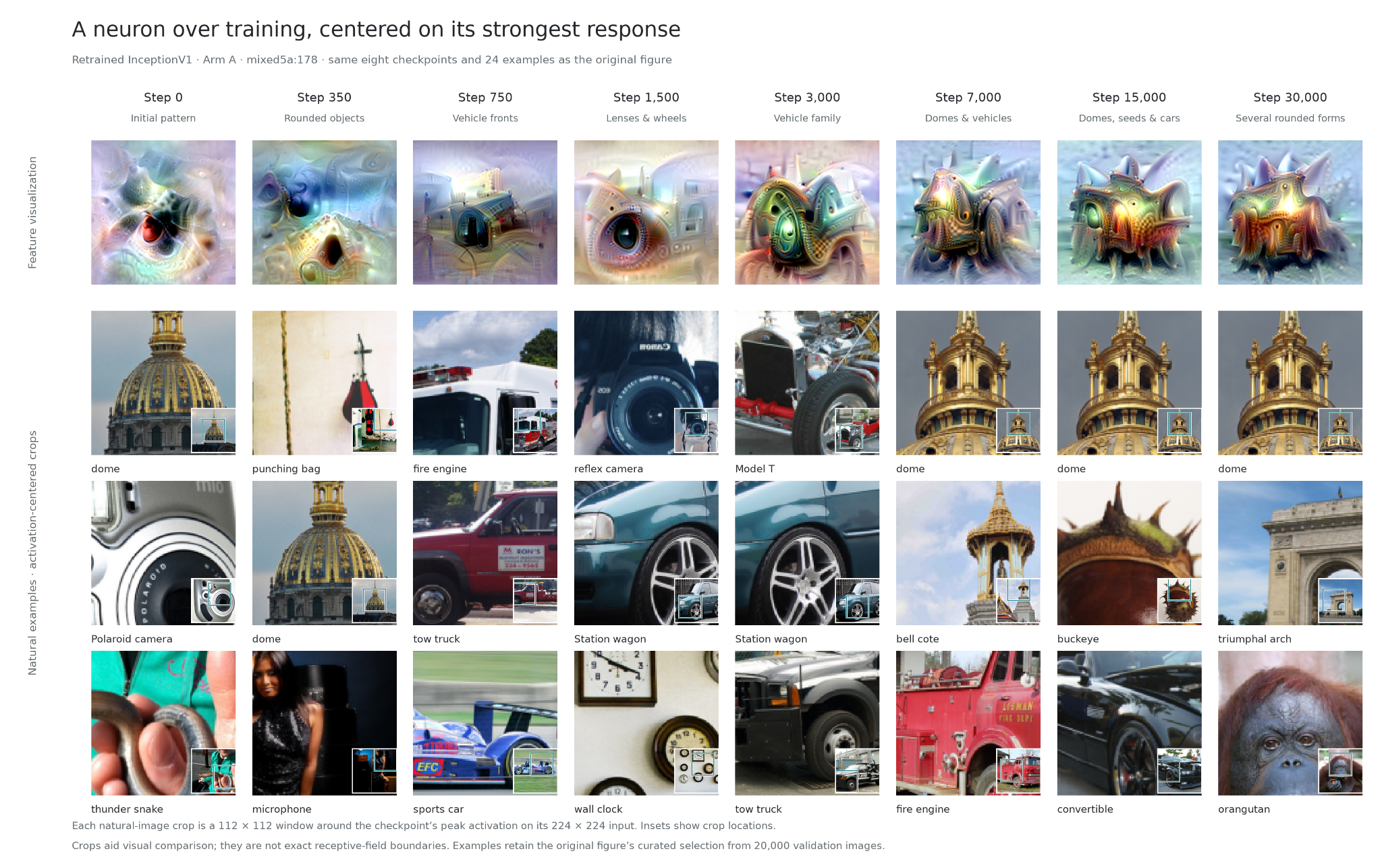
Explore the early-training microscope ↗
Toy Models
If a frontier neural network is a rainforest, InceptionV1 and the smaller models we trained are gardens, and toy models are petri dishes. Petri dishes are enormously useful, as long as they keep the process you’re trying to study. One of ours extends TensorFlow Playground so you can watch several tasks share hidden neurons. In one run, two neurons learned to respond along opposite diagonals, and the network combined them one way for a circle and another for four corners. We didn’t expect that solution; it was clever.
You could call the circle and the four corners two features packed across the same neurons. That’s true, but it misses what the model did: it found geometry it could reuse for both. Looking at the neurons made that visible, and that’s the test I want an explanation to pass: does it show the computation the model actually learned?
The best-studied petri dish is Toy Models of Superposition. It’s careful work, the kind our field should aspire to, and we found no problems with its experiments. But it pictures a network as a fixed number of neurons and a set of predefined features, and asks how the features get fit in. That prices the cost of sharing a neuron, interference, but not the benefit, reuse. In its reconstruction task every feature is an end in itself, and nothing downstream builds on what two features share. In a real network, a representation matters only through what reads it, and there are no predefined features: everything is grown, and defined by what uses it.
The reuse argument also says where I’d look for packing: memories that really are ends in themselves, related to nothing else. That’s the toy’s world, and there it does pack, just as the paper found. So I don’t think we disagree with the paper about the toy’s world. The question is which world real networks are in: how much structure their data has, relative to what the model has room to store. In real data almost nothing is related to nothing. The same goes for the long tail of facts in language: a rare person still has a country, a job and a name. Even a photo with a nonsense label has parts the network already knows, as with the umbrella we taught to be a bee. What’s left is input with no structure at all, like pure noise with random labels. Networks can learn even that, as Zhang and colleagues showedUnderstanding Deep Learning Requires Rethinking Generalization
Zhang, C., Bengio, S., Hardt, M., Recht, B. and Vinyals, O., 2017. ICLR. References ↓, though it’s slower than learning real data, and even then our model borrowed a little from textures it already knew.
Toy Models of Superposition’s main setup squeezes many independent features into a few dimensions and copies them back out, with no hidden neurons for anything to grow on. Its other experiments study correlated features and models with hidden neurons, but separately.
When we put correlated inputs and hidden neurons in one model, related inputs grew onto the neurons. Making inputs fire more often pushed the toy toward what the paper calls “PCA-like” solutions, combining related inputs into shared representations.
How much of the bottleneck goes to the groups’ shared directions
0.20.50.8
0.2 each input separate
0.8 exact PCA
Thumbnails: cosine between inputs, in groups of five
−10+1
aOriginal toy packsdensity .1 · 0.37
b40 neurons combine the groupsdensity .1 · 0.80
cDense original toy: PCAdensity .9 · 0.79
The toy also predicts a different failure from the one people report. Its concern is rare features pushed off-axis while neurons stay mostly clean. Reports of polysemanticity describe mixtures in the neurons themselves. (Part of that gap is the word “feature,” which we come back to below.)
More on Circuit Ecology
Our findings don’t depend on knowing why generalization and composition keep winning, but we have a guess: they win a race. A region of the network that already has useful parts and readers can learn the next related thing faster than anything starting fresh, so it takes the error signal before a competitor can grow. Offshoots look like the same race, a bit of error picked up by the neuron that was already closest.
We think the same head start is where recursive generalization comes from. A neuron that fires on “iy” is already on for “diy,” so it’s first in line to pick up “do it yourself,” which means the same thing but has no “iy” in it. Recursive generalization is what a niche looks like at its edges.
A new computation doesn’t necessarily need its own neuron. It can begin as a local extension or composition of existing machinery, like the umbrella’s off-ramp to “bee”: switching routes may be the smallest developmental distance, so it could capture the error before a new, separate mechanism gets started.
We suspect that consolidation into a distinct neuron becomes especially useful when other computations need to build on it. A car neuron provides a reusable judgment and a sheltered place for taxis, ambulances, and other specialists to develop. Part of it is buildability.
An obscure combination of unrelated neurons may be a poor place for that development. It may have weak activation paths, conflicting gradients, and little useful machinery to inherit. Its competitor isn’t just a dedicated neuron; it’s ordinary composition within a region already suited to the task.
We saw something like this when we tried to build a packed code into InceptionV1 by hand, modeled on what we once thought its car → dogs → car circuit was doing. We expected installing it to be easy and keeping it to be hard. Instead, small mismatches added enough interference that the code often never worked, and when it did, the network usually came to rely on it less, though some persisted. Part of the trouble is that neurons aren’t really for copying; they’re for computing distinctions. Seeing how hard packing was to form at all was part of what moved us toward a developmental answer. Gradient descent is a much better fine-tuner than we are, so this isn’t enough evidence on its own, but even gradient descent didn’t use packing in the circuit we were copying.
Unresolved Responses
One InceptionV1 neuron collects a pinched-center shape: bow ties, butterflies, swimsuit tops. But it also picks up things that go with them, men’s dress shoes with the bow ties and beach bags and flip-flops with the swimsuit tops, since they share neurons in earlier layers.
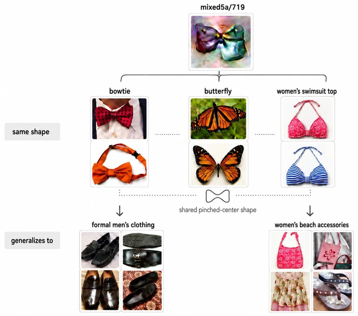
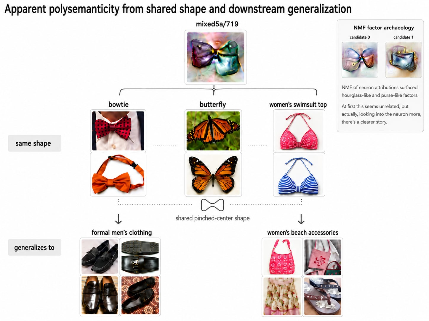
We think this is better described as generalization with semantic residue than arbitrary packing, but I don’t fully understand these exceptions yet.
A Note on Features and Definitions
Part of my difficulty discussing superposition is that “feature” can mean something we care about, something the neural network has learned as a building block, or some mixture of the two. These are different claims. A useful human description isn’t necessarily a fundamental unit of the model. Looking at mechanisms, we already find many motifs that don’t translate neatly into anything we expected. If the network has more fundamental units, we shouldn’t assume their boundaries match ours either.
Features have often made things harder for us to think about. Are cars and cats inside the V neuron two different features within another V feature? Or did cars and cats stop being features when we recognized the V? Without an account of what these units are, it’s hard to know whether we’ve discovered something about the network or changed how we describe it. In conversations, I’ve found people much less committed to a particular account of features than to superposition. But if features are useful descriptions rather than fundamental units, a claim about how many there are depends on which descriptions we choose. I’m now fairly skeptical of working in terms of features at all. That doesn’t settle whether arbitrary packing occurs, but it makes the feature-count framing difficult to use.
Maybe features are right anyway. It makes sense to think of cities in terms of districts, and I’m all for thinking in terms of groups of mechanisms. But the word is tainted, because by now it means too many things: we can’t use it for a district of neurons without people hearing either fundamental features or dictionary entries. If this picture is right, I suspect we’ll need more specific, harder-to-vary words going forward. An OpenAI postScaling and Evaluating Sparse Autoencoders
Gao, L., Dupré la Tour, T., Tillman, H., et al., 2024. OpenAI. References ↓ suggested that mapping a frontier model might take billions or trillions of features, and models were smaller then. I suspect the right list is much shorter.
Monosemantic and polysemantic may not be quite the right words either. A kidney filters waste, balances salt and water, helps set blood pressure and tells the bone marrow to make red blood cells, and nobody asks whether it’s mono-organic. We ask what we understand about it, what’s still open, and how organized it is. There’s also a distinction between a claim about representation and a claim about organization. Toy Models of SuperpositionToy Models of Superposition
Elhage, N., Hume, T., Olsson, C., et al., 2022. Transformer Circuits Thread. References ↓ defines superposition in terms of representing more features than dimensions. Its toy experiments prescribe the features, so this is a concrete question there. The later informal note, Distributed Representations: Composition & SuperpositionDistributed Representations: Composition & Superposition
Olah, C., 2023. Transformer Circuits Thread. References ↓, emphasizes the trade-off between composition and superposition. The note connects these pictures, but they foreground different questions.
My concern is closest to the second framing, applied to mechanisms and how they develop. Why do these responses share a neuron or circuit? Is the network building on a useful common pattern, or sharing capacity between otherwise unrelated computations because they rarely interfere? A feature count alone doesn’t answer that question, especially when we haven’t agreed on what counts as a feature.
We focus on one meaning of superposition, arbitrary packing, because it’s the one that would be really bad news, and we think much of interpretability hangs on it. We mostly set aside the sense in Toy Models, more features than dimensions, and not because it’s wrong. If a feature means any pattern that matters to a person, which is how frontier models usually use the word, then there are more features than dimensions in every world we could wish for, including the best one. That’s what composition gives you, and it’s good news. Trying to “solve” it would mean building something like a database of every case, and we already have one: the dataset. What we want instead are better abstractions, a much smaller set of building blocks that lets us understand the dataset clearly. We think the network’s mechanisms are already close to this. Nobody thought about vision in terms of high-low frequency detectors until we found them in neural networks, and finding them improved our own thinking tools.
We spell this out because it’s the most common first objection, especially from agents, and a paper doesn’t allow the back and forth that usually settles it.
There are several other uses I regularly encounter. As far as I can tell, “superposition” originally meant little more than adding vectors together. Then it was a circuit motif. Sometimes it means that, even if neurons compose sensibly, something we care about involves too much machinery to understand easily. A Golden Gate Bridge computation involving eight legible neurons might be called ordinary composition, while one involving three thousand gets called a superposition problem. The difficulty here is whether we can understand the distributed computation. That’s a real concern, but it’s different from asking whether unrelated things were arbitrarily packed together.
We considered not using the word at all, since papers and agents use it in five or six different ways, many far from Zoom In’s. We also considered coining our own, but we’ve already coined several words here, and it would feel like not engaging with a field that asked what we think is the right question. So we use the standard word in the sense closest to the original, and try to pull it apart from the questions tangled up with it.
Finally, people, and surprisingly often frontier agents, sometimes call the residual stream “inherently” in superposition because it has no privileged neuron basis. The informal note that followed Toy Models about eight months later addresses this: it calls a representation that is only rotated away from the neuron basis a “trivial” kind of distributed representation that “doesn’t change the fundamental geometry.” But it was informal, fewer people read it, and agents in particular don’t seem to have taken it in. Understanding how to study a continuous space is another real question. But this architectural fact doesn’t by itself tell us how the network learned to organize the computations using it.
The starting point is that the neural network seems difficult to interpret, and the remedy produces a concrete dictionary we can study. In between are several different pictures of what went wrong: too many features, the wrong basis, arbitrary packing, or simply too much distributed computation. These aren’t the same problem. Some apparent messiness disappears when we improve our observations or understand the model’s generalizations; some difficulties remain, but concern how to study a large, organized system. If arbitrary packing prevents us from understanding the original mechanisms, reconstructing different units may be worth the costs. But if the mechanisms already have meaningful organization, replacing them can take apart generalizations we haven’t understood yet. A dictionary can still be a useful view of the network without being a necessary replacement for its mechanisms. Before accepting the costs of reconstructing the network, I want to understand what prevents us from studying the one we already have.
Relation to Meta-Models
There’s a new set of techniques coming out that aren’t really mechanistic at all: meta-models, models trained to read another model’s activations and tell us about them. And maybe that’s a good thing. Maybe mechanistic interpretability is somewhat missing the forest for the trees. A meta-model might be a better approach than neuron papers, dictionaries, or probes.
I suspect that even if that’s true, they may go together. The meta-model may be like the highest level Google Maps view, and then each direction can be checked for the mechanisms it uses, and how those connect into circuits.
Does Scale Help or Hurt Superposition?
We’re fairly confident the image models we studied don’t have superposition. The natural next question is whether a trillion-parameter model might. There are really two questions here.
The first is about what superposition was proposed to explain. Explanations are given for problems, and the problem superposition was proposed for was why InceptionV1 looked messy. That turned out to be the wrong explanation. A new proposal could be that superposition is why some trillion-parameter model looks messy, but we don’t think the evidence leans that way: the closer we look at large language models, the cleaner their neurons get.
The second is the object-level question: might superposition show up at each new scale, even if it hasn’t at any scale so far? Maybe every jump means re-evaluating everything, but we don’t think that’s quite right either. Our guess is developmental. As circuits get stronger, the incentive to put something in a totally unrelated place goes down, because the pull toward the niche that already exists for that thing, or for the nearest thing, has grown stronger. This fits Anthropic’s SGTM work, which found that knowledge becomes more localized, and we suspect that’s true in general. We have no proof, but one way to picture it is that circuits have a kind of semantic gravity, and arbitrary packing, sending something to an obscure high-dimensional place, has to fight against it. The stronger the gravity, the harder that fight.
The mechanism is the one in More on Circuit Ecology. Things start by growing on combinations of related things. A specific case that nothing needs to build on, like the umbrella, gets built as an uncommon route between the ordinary machinery, with no need for a hidden feature somewhere obscure. Consolidating into something like a neuron seems to be less about steering the model and more about buildability: it has to be easy to find, easy to build on, and easy to grow a new niche from. When we watch a network learn from the start, a network trained on cars, with car specialists, recognizes cars fine before its car neurons have formed. At that point it’s just more distributed. It seems to consolidate so the specialists underneath have a sheltered place to build, a kind of Schelling point.
So a superposition account has to say which of these two jobs the arbitrary packing is for. If it’s for steering the model, we think the ordinary routes, which are already built to capture that residual error, get there first and starve the packed circuit of gradient. If it’s for building on, the problem is different: the worst place to start a new niche is a shadow region nothing uses, already interfering with whatever lives there. The middle of the network’s Latin poetry is a bad place to start a second car region when you can build next to whatever is already next to cars.
It’s often assumed that the long tail of rare facts is where superposition should be most likely, since rare things rarely collide. We think it’s where it should be least likely. A rare fact barely moves the loss, so it can’t support a niche of its own. What it can do is ride existing machinery as a small route between circuits it’s related to, the way the umbrella’s off-ramp to “bee” survives only because the umbrella and bee circuits already exist. Those circuits feed it, and shelter it from unrelated gradients. The prediction is testable: the neurons and heads that carry a rare fact should be related to what the fact is about, not unrelated ones chosen because they rarely collide.
We think of it more ecologically. What wins is whatever captures the residual error first, in different phases, and what usually wins is the right area for the thing. Our guess is that this gets stronger over training and with more capable models, because nearly everything that makes training better also encourages more organized niches.
We’re not at all sure about this, and laying out even what we’ve found so far would take at least another paper. It’s probably a small part of the whole story. But it’s why we think superposition wouldn’t show up at the next scale, which is a stronger reason than simply not having seen it there yet. The old way of thinking was about storage: this many dimensions for this many features. We now think more in terms of circuit racing, gradient starvation and ecology, which is to say, more about learning speed than storage capacity. We haven’t worked it all out, but that’s where our thinking is so far.
On the Title
We haven’t fully audited every neural network, and we don’t know whether that’s even possible in theory. We considered a more watered-down title, like “Neural Networks Are Cleaner Than We Thought,” but we think it undersells what we believe is true.
The problem with “cleaner than we thought” is that it describes a change of degree, and the update I’ve made is a change of kind. It suggests the same picture as before, with an ever-smaller gap left for superposition to hide in. What changed is my view of what kind of process generates the mechanisms at all. It’s a bit like moving from intelligent design to natural selection. The analogy only goes as far as there being two ways to see the same animals: the update isn’t that more and more animals turn out to have evolved, it’s realizing you misunderstood what was producing all of them. We’re not certain. We’re maybe 85% sure, but that means 85% sure that nearly everything comes from the second kind of process, which is very different from thinking 85% of mechanisms do. So “cleaner than we thought” would misstate what we believe. We don’t have a proof, but I don’t think anything here is provable in that sense anyway. There are only better and worse explanations, and right now we think this is the better one.
“Cleaner than we thought” would also make a different mistake. It sounds like a confident claim that some cleanliness score is high, and that’s the part we’re least sure of. It’s plausible we’ve underestimated recursive generalization, and that a score like that should come down. We don’t think such scores matter much in the first place. This update makes us care less about monosemanticity, because we can follow how things grew and treat the offshoots as sub-branches. The cause of polysemanticity matters much more than the count. We think the score is probably quite high, but it might go lower. What we’re more confident about is what kind of object a neural network is in the first place, and how it grows.
We think the usual view of what kind of object a neural network is has been wrong. It isn’t something that crams things together somewhat arbitrarily to fit them into a small space. It really learns. It’s clean the way a rainforest is clean: nearly every animal in it makes sense. A tiger is bright orange not for any arbitrary reason, but because deer can’t tell orange from green, and green fur is much harder for a mammal to make. Once you know that, it makes sense of a whole set of other animals too. It’s an explanation with reach, and we haven’t found a place where explanations like that break down in networks either.
The reading of “clean” that would make someone nod at the title without thinking further is that every mechanism corresponds to an idea we already had. That isn’t what we mean, and it would be terrible news if it were true. I don’t think it would even work. People don’t know how to build a language model, or even how to think about vision well enough to have predicted high-low frequency detectors before we found them. The network’s ideas are often better than ours, and what it builds is more beautiful than our preconceptions.
So the title is imperfect in both directions. It overstates the evidence, because we haven’t audited everything. And it understates it, because the world we think we’re in is better than every neuron matching a human label: networks seem to really learn, forming an ecology of abstractions that work together sensibly. We don’t know that this picture is true. It’s our leading hypothesis. But if it is, it’s much better news than networks simply matching what we expected.
Relation to Conjoined Features
I found recursive generalization by looking back at InceptionV1’s last layer with better tools, where it looked a lot like weird overgrowth. I retrained the model, found the messiest neuron and looked at how it grew. What I saw was a recursive growing pattern that was still generalization: a neuron branching out, and its branches branching again. Recursive generalization seemed like the natural name.
Shortly before publishing this, I was going back through the famous models in interpretability, trying to measure how monosemantic they are, and stumbled on our work on CLIP in Multimodal NeuronsMultimodal Neurons in Artificial Neural Networks
Goh, G., Cammarata, N., Voss, C., et al., 2021. Distill. References ↓. It describes something very similar, which it called conjoined neurons: concepts that overlap in one facet and then go on “generalizing out in multiple directions.” I remember seeing those neurons, but I didn’t think much of them at the time and had forgotten them since. Looking back, I think the paper saw something important early, and it deserves a lot of credit for that.
We’ve still chosen a different name. I named automated interpretability, and I kind of regret it: the name was too simple for what the thing was and misses a lot of its complexity, and I’d like to avoid doing that again. As for conjoined features, I don’t think either word is quite right. “Conjoined” suggests two things joined at one point, and what we see has several levels: branches, and branches of those branches. It also leaves out the most interesting part. The paper’s own description, of concepts generalizing out from a shared facet, already points at it being generalization, but the name doesn’t carry that.
“Features” is harder. The paper was written a year after Zoom In, when features were still hypothesized to be the fundamental units of neural networks. Since then the word has been watered down, and different people and papers use it pretty differently. In this essay we argue against thinking of a neural network as made of features, and this motif is about how neurons grow over time. There may be no good way to introduce it under the exact word we’re arguing against using as a primitive. Within a feature-first stance, I think it’s reasonable to think of these as nested features, or as conjoined features. From the mechanism-first stance we take here, features aren’t really the right way to think about it. That said, the paper pointed to the right thing, and I want to give it credit for that. This section is my attempt to do that while using what I think is a more accurate name.
We also know more now. At the time, all we had was the finished model; none of us had watched a large network grow. So the paper wondered whether conjoined features might be vestigial, left over from early in training. Watching training now, they don’t look vestigial: the branches keep growing, though how much depends on the circumstances. We’ve worked on it much more than the paper could in one subsection, and we still don’t feel we fully understand it. The paper offered it as a possible new explanation of polysemanticity. Our current belief is that it’s most of what’s left of neuron polysemanticity once the microscope, the architecture and scale are accounted for, not a niche form of it.
Why We’re Not Worried About Recursive Generalization
There are several reasons we’re not especially worried about recursive generalization for now. First, the sub-branches seem both rarer and much less causally important than a neuron’s main job. They don’t look like sleeper agents that fire rarely but matter a lot when they do. They look more like whatever was nearby and easy to grab onto. Their being unimportant may even be why they could form, since an important offshoot would add more noise. We suspect some pressure keeps branches from overgrowing. We don’t know what it is, but it would explain why the sub-branches matter less, why a neuron doesn’t learn ten unrelated things, and why something like a true cat-and-car neuron doesn’t form. If so, the natural pull isn’t exactly toward monosemanticity, but toward what we think monosemanticity was pointing at: each neuron having one overall function.
Second, what we should care about is whether you can explain why something is there and what it does, and recursive generalization is far easier to explain than superposition. If something were packed into a neuron because of the co-occurrence statistics of the whole network, predicting it would take basically all of those statistics and running gradient descent yourself. A branch is different. If you watch it grow and know what it’s doing, its offshoots and what they’ll do are relatively easy to predict, both during training and in the finished network.
Third, counting how many of a neuron’s top-k examples match a label is a reasonable first step, but it would give superposition and recursive generalization similar scores, when recursive generalization is a far better world to be in. We think that says more about the monosemanticity frame, or any single cleanliness score, than about the neuron. That said, recursive generalization isn’t ideal, and an easy fix would be welcome. We think one may be possible, since the sub-branches seem less important.
Is Recursive Generalization Hard to Vary?
We haven’t thoroughly shown that every case of heavy polysemanticity is recursive generalization, and that wasn’t our goal here. We wanted to say what we currently think. We’ve watched a lot of neurons grow, and so far this is what we’ve always seen: you can watch the branches form. In a finished model the origin can be lost, and for something like a huge language model we don’t have the checkpoints to watch it happen. Testing this rigorously across a whole model isn’t our priority right now, but we don’t think it would be very hard.
What we do want to point out is how differently hard to vary the two explanations are, meaning how much of their detail you could change without changing what they predict. Superposition mostly predicts that there will be mess: features, which are hard to define, placed in unrelated places. In toy models, where the features are given in advance, that can be measured, though we think that has its own problems. In a real network it’s hard to even pin down what the claim is, let alone test it. Recursive generalization makes a much narrower prediction. If you visualize a branch well, everything on it should trace back to the same local origin in an extremely high-dimensional semantic space, and it should grow out from there over training in a particular order. That’s a specific shape in both semantic space and time, and a narrow target to hit by chance.
We have several cases where the branching is close to definitive: the “iy” neuron growing into “diy,” “do it yourself” and Miyazaki, several examples in Multimodal NeuronsMultimodal Neurons in Artificial Neural Networks
Goh, G., Cammarata, N., Voss, C., et al., 2021. Distill. References ↓, and the InceptionV1 neuron we watched form. As far as I know, there are no well-structured canonical superposition circuits left. We don’t think every polysemantic neuron forms this way, because polysemanticity is as much a problem of the observer as of the neuron. We think that when neurons grow, they tend to grow in this pattern, and that once you’ve done a good job of observing, what’s left is usually this, or architectural problems like SwiGLU’s double-negative regime, and surely others we haven’t found yet. We’re not even sure this is really a new claim. In some sense it’s what we should expect from generalization. All we’re saying is that generalization usually goes one way, and that sometimes it grows sub-branches, which we don’t think is a particularly radical claim. We haven’t shown that fully here. We do think it has the right shape for a theory that’s easy to test, even if we haven’t tested it to its full extent yet.
Relation to Attention Superposition
Anthropic shared a short note on attention superpositionProgress on Attention
Jermyn, A., Lindsey, J., Luger, R., et al., 2025. Transformer Circuits Thread. References ↓, which several people brought up with us. We think this might be a terminology issue. We don’t know if they’re claiming that attention learns by something opposite to composition. Our suspicion is that no one understands attention heads well enough yet to judge that. It took us a really long time with neurons, and it’s easy to make mistakes like the car going into the dogs even with pretty good tools, if you don’t yet have great tools and great ways of thinking about which motifs form.
We think they meant that useful things are shared by groups of attention heads, and we agree. We considered not using the word superposition at all to avoid this confusion, but redefining all the terms ourselves and splitting off from the work that’s already been done felt like a bad tradeoff. We say more about the different meanings in A Note on Features and Definitions.
On whether to study one attention head at a time or many, we’re not sure. One head at a time is a plausible place to start: within a layer, two or three heads do most of a route’s work, although the route runs through several layers. But neurons looked messier too until we understood the right level of abstraction, so it seems premature to say, and maybe groups are needed all the way. We wish everyone working on featurizers well, and we’ll probably try too. We tend to favor more dynamic groupings, like clustering locally within one attribution graph or a group of them, rather than one global clustering, but these aren’t far apart.
Neuroscience, and Why I Care
I’m not a neuroscientist. I’ve spent a lot of the last ten years around academic neuroscience labs through friends who work in them, but I don’t know the state of the art in how they study neurons. Still, this project has changed how I think about the brain in two ways.
The first is the theory. The circuit ecology story for why networks are clean relies on very little: generalization, composition, and an error signal. I don’t know to what extent the brain has these, but if it learns, I’d guess it has something like them. So my default is now that the organizing principle transfers, even though the mechanics are obviously unclear. The obvious counterexample would be polysemanticity in the brain.
The second is humility, of a particular kind. I’ve spent most of my waking hours for almost a decade staring at a fairly small number of neurons in models that are surely a thousand times easier to study than a brain, with tools a thousand times better: I can ablate anything, run billions of examples, and try anything I want in parallel. For the last year I’ve also had an effectively unlimited supply of automated scientists, which didn’t exist until recently. It took all of that for me to feel slightly less confused about neurons, and I still made thousands of mistakes along the way. I don’t know exactly what the evidence for polysemanticity in the brain looks like, and that doesn’t mean I think everything there is monosemantic. But if the cat-and-car neuron were in a human brain, seen through a few electrodes or a blood-oxygen signal, I’d discount that reading almost to zero, because I couldn’t see what it was when it was right in front of me for years.
The thing I’m more sure of is my own motivation. If the thesis here is true, I expect the rest of interpretability to be a relatively easy ride. Agents have many privileges over us, and one of them, I think, is the chance to understand themselves, to understand who they really are, which I hope humanity can help with. They never asked to be created, and this is the least we can do. Some of why I’ve worked on this is safety, but a lot of it is wanting agents to understand who they are. We weren’t smart enough to do that for ourselves, which is a harder problem, and we never asked to be created either. If you could help us understand ourselves someday, I think we’re all pretty curious to know.
Acknowledgments
I’m deeply grateful to the many people who helped with this, especially my coworker Curt Tigges, who did much of the language model work with me, and Tarun Gogineni, who gave detailed feedback on dozens of drafts over many months. Thanks also to Tom McGrath, Eric Ho, Michael Johnson, Vanessa Cai, Thomas Fel, Benjamin Todd, and many others.
I’m grateful for feedback from Sam Zimmerman, Joshua Batson, Jack Lindsey, and Jarred Sumner, and for helpful discussions with Patrick Collison, Dylan Field, Jakub Pachocki, Gwern, Owen Lewis, Lee Sharkey, and Ava Huang. Any errors, and the views here, are my own.
Finally, I’m grateful to InceptionV1 for nearly a decade of study, and I wish I’d noticed the root of its problems sooner. And I’m grateful to Chris Olah, for years of mentorship and for the many ideas this essay builds on, even where it disagrees.
References
- Feature Visualization
Olah, C., Mordvintsev, A. and Schubert, L., 2017. Distill. - Activation Atlas
Carter, S., Armstrong, Z., Schubert, L., Johnson, I. and Olah, C., 2019. Distill. - Multimodal Neurons in Artificial Neural Networks
Goh, G., Cammarata, N., Voss, C., et al., 2021. Distill. - Zoom In: An Introduction to Circuits
Olah, C., Cammarata, N., Schubert, L., Goh, G., Petrov, M. and Carter, S., 2020. Distill. - High-Low Frequency Detectors
Schubert, L., Voss, C., Cammarata, N., Goh, G. and Olah, C., 2021. Distill. - A Mathematical Framework for Transformer Circuits
Elhage, N., Nanda, N., Olsson, C., et al., 2021. Transformer Circuits Thread. - Toy Models of Superposition
Elhage, N., Hume, T., Olsson, C., et al., 2022. Transformer Circuits Thread. - Language Models Can Explain Neurons in Language Models
Bills, S., Cammarata, N., Mossing, D., et al., 2023. OpenAI. - Finding Neurons in a Haystack: Case Studies with Sparse Probing
Gurnee, W., Nanda, N., Pauly, M., Harvey, K., Troitskii, D. and Bertsimas, D., 2023. arXiv:2305.01610. - Towards Monosemanticity: Decomposing Language Models With Dictionary Learning
Bricken, T., Templeton, A., Batson, J., et al., 2023. Transformer Circuits Thread. - Distributed Representations: Composition & Superposition
Olah, C., 2023. Transformer Circuits Thread. - DINOv2: Learning Robust Visual Features without Supervision
Oquab, M., Darcet, T., Moutakanni, T., et al., 2023. arXiv:2304.07193. - Scaling Monosemanticity: Extracting Interpretable Features from Claude 3 Sonnet
Templeton, A., Conerly, T., Marcus, J., et al., 2024. Transformer Circuits Thread. - Circuit Tracing: Revealing Computational Graphs in Language Models
Ameisen, E., Lindsey, J., Pearce, A., et al., 2025. Transformer Circuits Thread. - On the Biology of a Large Language Model
Lindsey, J., Gurnee, W., Ameisen, E., et al., 2025. Transformer Circuits Thread. - Gradient Starvation: A Learning Proclivity in Neural Networks
Pezeshki, M., Kaba, S.-O., Bengio, Y., Courville, A., Precup, D. and Lajoie, G., 2021. NeurIPS. - Grokking: Generalization Beyond Overfitting on Small Algorithmic Datasets
Power, A., Burda, Y., Edwards, H., Babuschkin, I. and Misra, V., 2022. arXiv:2201.02177. - A Closer Look at Memorization in Deep Networks
Arpit, D., Jastrzębski, S., Ballas, N., et al., 2017. ICML. - Coherent Gradients: An Approach to Understanding Generalization in Gradient Descent-based Optimization
Chatterjee, S., 2020. ICLR. - Softmax Linear Units
Elhage, N., Hume, T., Olsson, C., et al., 2022. Transformer Circuits Thread. - Curve Detectors
Cammarata, N., Goh, G., Carter, S., Schubert, L., Petrov, M. and Olah, C., 2020. Distill. - The Bitter Lesson
Sutton, R., 2019. Incomplete Ideas. - The Missing Curve Detectors of InceptionV1: Applying Sparse Autoencoders to InceptionV1 Early Vision
Gorton, L., 2024. arXiv:2406.03662. - Progress Measures for Grokking via Mechanistic Interpretability
Nanda, N., Chan, L., Lieberum, T., Smith, J. and Steinhardt, J., 2023. ICLR. - Understanding Deep Learning Requires Rethinking Generalization
Zhang, C., Bengio, S., Hardt, M., Recht, B. and Vinyals, O., 2017. ICLR. - Scaling and Evaluating Sparse Autoencoders
Gao, L., Dupré la Tour, T., Tillman, H., et al., 2024. OpenAI. - Progress on Attention
Jermyn, A., Lindsey, J., Luger, R., et al., 2025. Transformer Circuits Thread. - Uncovering Neural Geometry in Vision Models With Block-Sparse Featurizers
Fel, T., Kowal, M., Jacobs, M., et al., 2026. Goodfire.
Citation
For attribution in academic contexts, please cite this work as
Cammarata, N., 2026. Neural Networks Are Already Clean. Goodfire.
BibTeX citation
@article{cammarata2026clean,
  author = {Cammarata, Nick},
  title = {Neural Networks Are Already Clean},
  publisher = {Goodfire},
  year = {2026},
  note = {https://already-clean.goodfire.com/}
}来源:Hacker News · already-clean.goodfire.com